Toda Lattice

The Toda lattice is a prime example of an completely-integrable system, i.e. a Hamiltonian system evolving in $\mathbb{R}^{2n}$ that has $n$ Poisson-commuting invariants of motion (see [3]). It is named after Morikazu Toda who used it to model a one-dimensional crystal [5].

The Hamiltonian of the Toda lattice takes the following form:

\[ H(q, p) = \sum_{n\in\mathbb{Z}}\left( \frac{p_n^2}{2} + \alpha e^{q_n - q_{n+1}} \right).\]

In practice we work with a finite number of particles $N$ and impose periodic boundary conditions:

\[\begin{aligned} q_{n+N} & \equiv q_n \\ p_{n+N} & \equiv p_n. \end{aligned}\]

Hence we have:

\[ H(q, p) = \sum_{n=1}^{N-1} \left( \frac{p_n^2}{2} + \alpha e^{q_n - q_{n+1}} \right) + \frac{p_N^2}{2} + \alpha e^{q_N - q_1}.\]

We can model the evolution of a thin pulse in this system:

problem = GeometricProblems.TodaLattice.hodeproblem()
sol = integrate(problem, ImplicitMidpoint())

time_steps = (0, 200, 400, 600, 800, 1000, 1200)
p = plot()
for time_step in time_steps
    plot!(p, sol.q[time_step, :], label = "t = $(sol.t[time_step])")
end

p

As we can see the thin pulse separates into two smaller pulses an they start traveling in opposite directions until they meet again at time $t\approx120$. But it is important to note that the right peak at time $120$ is below the one at time $0$. This is not a numerical artifact but a feature of the Toda lattice!

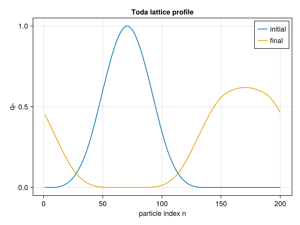
Library functions