Three Body Problem

using GeometricProblems.ThreeBody: hodeproblem
using GeometricIntegrators: ImplicitMidpoint, integrate
using CairoMakie
using LaTeXStrings

morange = RGBf(255 / 256, 127 / 256, 14 / 256)
mred = RGBf(214 / 256, 39 / 256, 40 / 256)
mpurple = RGBf(148 / 256, 103 / 256, 189 / 256)
mblue = RGBf(31 / 256, 119 / 256, 180 / 256)
mgreen = RGBf(44 / 256, 160 / 256, 44 / 256)

pr = hodeproblem(; tstep = .2)
sol = integrate(pr, ImplicitMidpoint())
first_body = zeros(2, length(sol.s.q))
second_body = zeros(2, length(sol.s.q))
third_body = zeros(2, length(sol.s.q))

for index in axes(sol.s.q, 1)
  data_for_present_index = sol.s.q[index]
  first_body[:, index + 1] = data_for_present_index[1:2]
  second_body[:, index + 1] = data_for_present_index[3:4]
  third_body[:, index + 1] = data_for_present_index[5:6]
end

fig = Figure()
ax = Axis(fig[1, 1])
scatter!(ax, first_body, color = mred)
lines!(ax, first_body, color = mred, linestyle = :dash)
scatter!(ax, second_body, color = mblue)
lines!(ax, second_body, color = mblue, linestyle = :dash)
scatter!(ax, third_body, color = mgreen)
lines!(ax, third_body, color = mgreen, linestyle = :dash)

scatter!(ax, first_body[:, 1]', color = :black, label = L"t = 0")
scatter!(ax, second_body[:, 1]', color = :black)
scatter!(ax, third_body[:, 1]', color = :black)
axislegend(position = :rb)

fig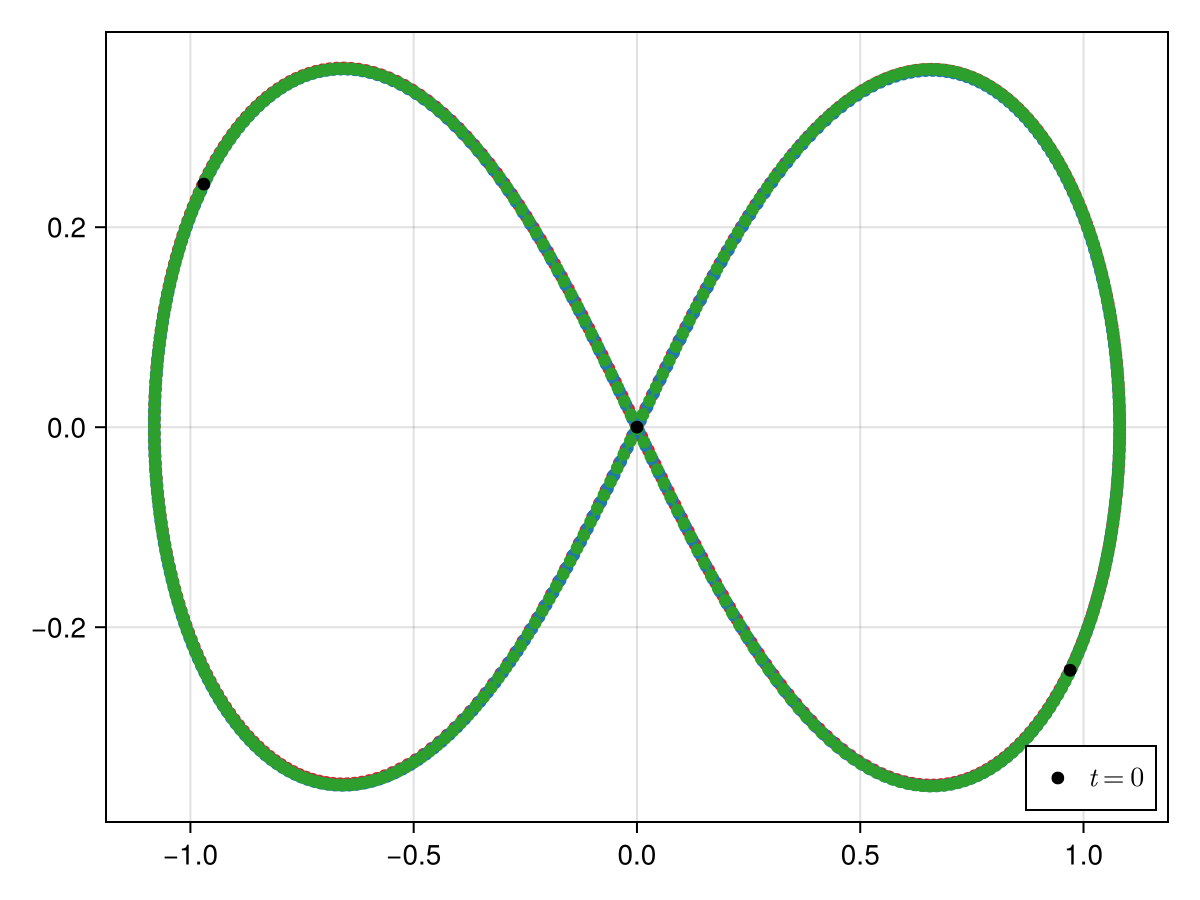

Library functions

GeometricProblems.ThreeBody — Module

ThreeBody

System parameters:

m₁: mass of body 1
m₂: mass of body 2

source

GeometricProblems.ThreeBody.G — Constant

Constant taken from [5].

source

GeometricProblems.ThreeBody.default_parameters — Constant

Default parameters taken from [5].

source

GeometricProblems.ThreeBody.initial_conditions — Constant

Here we get 4096 trajectories that should be similar to the data used in [5].

source

GeometricProblems.ThreeBody.m₁ — Constant

Constant taken from [5].

source

GeometricProblems.ThreeBody.m₂ — Constant

Constant taken from [5].

source

GeometricProblems.ThreeBody.m₃ — Constant

Constant taken from [5].

source

GeometricProblems.ThreeBody.tspan — Constant

Range is taken from [5]. In that reference the integration is only done for ten time steps.

source

GeometricProblems.ThreeBody.tstep — Constant

Constant taken from [5].

source

GeometricProblems.ThreeBody._reshape — Method

Turn array into a vector.

source

GeometricProblems.ThreeBody.hodeproblem — Function

hodeproblem(q₀, p₀; tspan, tstep, parameters)

Hamiltonian version of the three-body problem

Constructor with default arguments:

hodeproblem(
    q₀ = [0.5877852522924731, 0.8090169943749475, 0.8090169943749475, 0.5877852522924731, 0.8090169943749475, 0.8090169943749475],
    p₀ = [0.5877852522924731, 0.8090169943749475, 0.8090169943749475, 0.5877852522924731, 0.8090169943749475, 0.8090169943749475];
    tspan = (0.0, 5.0),
    tstep = 0.5,
    params = (m₁ = 1.0, m₂ = 1.0, m₃ = 1.0, G = 1.0)
)

source

GeometricProblems.ThreeBody.lodeproblem — Function

lodeproblem(q₀, p₀; tspan, tstep, parameters)

Lagrangian version of the three-body problem

Constructor with default arguments:

lodeproblem(
    q₀ = [0.5877852522924731, 0.8090169943749475, 0.8090169943749475, 0.5877852522924731, 0.8090169943749475, 0.8090169943749475],
    p₀ = [0.5877852522924731, 0.8090169943749475, 0.8090169943749475, 0.5877852522924731, 0.8090169943749475, 0.8090169943749475];
    tspan = (0.0, 5.0),
    tstep = 0.5,
    params = (m₁ = 1.0, m₂ = 1.0, m₃ = 1.0, G = 1.0)
)

source

References

[5]: P. Jin, Z. Zhang, A. Zhu, Y. Tang and G. E. Karniadakis. SympNets: Intrinsic structure-preserving symplectic networks for identifying Hamiltonian systems. Neural Networks 132, 166–179 (2020).