Harmonic Oscillator

The equations of motion of a harmonic Oscillator with spring constant $k$ and mass $m$ are given by

\[m \, \ddot{x} (t) = - k \, x (t) , \qquad x(t_0) = x_0 , \qquad \dot{x} (t_0) = \dot{x}_0 .\]

Its solution is obtained as

\[x (t) = A \, \cos( \omega (t - t_0) - \varphi )\]

with the frequency $\omega = \sqrt{k / m}$, amplitude $A = x_0 \, \sqrt{1 + \dot{x}_0^2 / (m k x_0^2)}$, and phase $\varphi = \arctan(\dot{x}_0 / (m \omega x_0))$. The energy of the system is

\[E(x, \dot{x}) = \frac{m}{2} \dot{x}^2 + \frac{k}{2} x^2 .\]

Hamiltonian Formulation

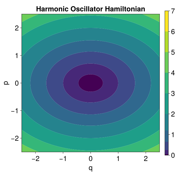
In canonical Hamiltonian coordinates $(q = x, \, p = m \dot{x})$, the Hamiltonian of the harmonic oscillator is given by

\[H(q, p) = \frac{1}{2m} p^2 + \frac{k}{2} q^2 ,\]

such that Hamilton's equations of motion read

\[\dot{q} = \frac{\partial H}{\partial p}(q, p) = \frac{p}{m} , \qquad \dot{p} = - \frac{\partial H}{\partial q}(q, p) = - k q , \qquad q(t_0) = q_0 , \qquad p(t_0) = p_0 .\]

and their solution is given by

\[q (t) = A \, \cos( \omega (t - t_0) - \varphi ) , \qquad p (t) = - \omega A \, \sin( \omega (t - t_0) - \varphi ) ,\]

with

\[A = q_0 \, \sqrt{1 + p_0^2 / (k q_0^2)} , \qquad \varphi = \arctan(p_0 / (\omega q_0)) .\]

Lagrangian Formulation

The harmonic oscillator derives from the regular Lagrangian

\[L(x, \dot{x}) = \frac{m}{2} \dot{x}^2 - \frac{k}{2} x^2 ,\]

whose Euler–Lagrange equation $\tfrac{d}{dt} \tfrac{\partial L}{\partial \dot{x}} - \tfrac{\partial L}{\partial x} = 0$ reproduces $m \ddot{x} = -k x$. The conjugate momentum is $p = \partial L / \partial \dot{x} = m \dot{x}$, and the Legendre transform $H = p \dot{x} - L$ recovers the Hamiltonian above.

Besides this regular Lagrangian, the module also provides a degenerate, first-order (phase-space) Lagrangian of the form $L(q, \dot{q}) = \vartheta(q) \cdot \dot{q} - H(q)$, which underlies the implicit/variational formulations (iodeproblem, lodeproblem, and their degenerate_ variants).

Dynamics

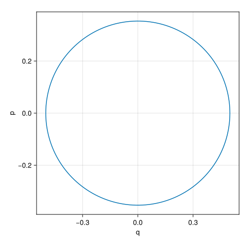
The harmonic oscillator is provided in many equivalent formulations, all describing the same dynamics and conserving the energy $H$: an explicit ODE (odeproblem), a partitioned/Hamiltonian system (podeproblem, hodeproblem), implicit and variational forms (iodeproblem, lodeproblem), a split ODE (sodeproblem), differential-algebraic forms (daeproblem, pdaeproblem, hdaeproblem, idaeproblem, ldaeproblem), and discrete Euler–Lagrange problems (deleproblem_midpoint, deleproblem_trapezoidal), together with the corresponding ensembles. Integrating the default Hamiltonian problem traces a closed trajectory in phase space:

Library