Pendulum

The mathematical pendulum is a canonical Hamiltonian system. In a unit system where gravity, mass and length are equal to one its Hamiltonian is

\[H(q, p) = \frac{p^2}{2} + \cos(q) ,\]

with angle $q$ and conjugate momentum $p$, giving the equations of motion

\[\dot{q} = p , \qquad \dot{p} = -\sin(q) .\]

We take the problem from GeometricProblems.jl. As for the harmonic oscillator, we integrate the canonical HODEProblem with the symplectic partitioned method PartitionedGauss, and the plain ODEProblem (state $[q, p]$) with the symplectic ImplicitMidpoint method and the non-symplectic explicit Runge-Kutta method RK4. The plotting functions plot_loop, plot_surface and plot_invariant come from the package's Makie extension, activated by loading CairoMakie.

using PoincareInvariants
using GeometricIntegrators
using GeometricProblems.Pendulum
using CairoMakie

probh = hodeproblem([0.0], [0.0]; timespan = (0.0, 5.0), timestep = 0.2)  # canonical
probo = odeproblem([0.0, 0.0];   timespan = (0.0, 5.0), timestep = 0.2)   # plain ODE

First invariant

The first invariant is the loop integral of the canonical one-form,

\[I_{1} = \oint_{\gamma} p \, dq ,\]

the area enclosed by the closed curve $\gamma$. We use a circle of radius $r = 1/2$ centred at the stable equilibrium $(q, p) = (\pi, 0)$ (recall that for $H = p^2/2 + \cos q$ the point $q = 0$ is the unstable equilibrium).

r = 0.5
init1 = ϕ -> (π + r * sinpi(2ϕ), r * cospi(2ϕ))

pi1 = CanonicalFirstPI{Float64, 2}(500)

sol1_pg = integrate(PIEnsembleProblem(probh, pi1, init1), PartitionedGauss(1))
sol1_im = integrate(PIEnsembleProblem(probo, pi1, init1), ImplicitMidpoint())
sol1_rk = integrate(PIEnsembleProblem(probo, pi1, init1), RK4())

The loop is transported around the equilibrium and progressively sheared by the flow, yet the enclosed area (the first invariant) is preserved:

plot_loop(sol1_pg; xlabel = "q", ylabel = "p")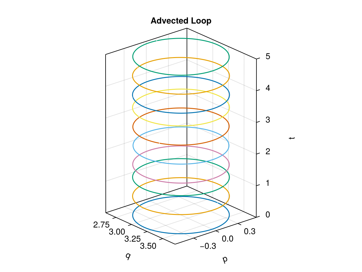

plot_invariant(pi1, sol1_pg; title = "PartitionedGauss")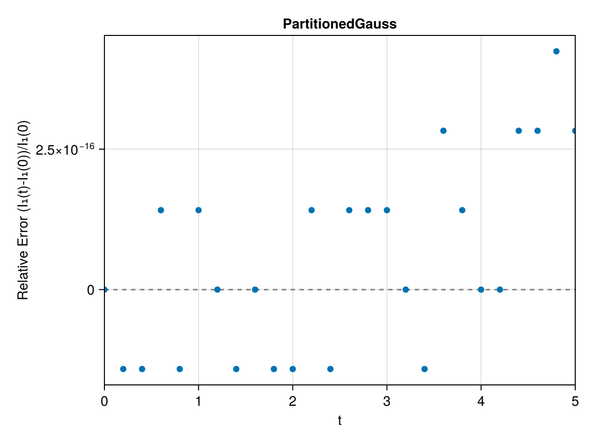

plot_invariant(pi1, "ImplicitMidpoint" => sol1_im, "Explicit Runge-Kutta-4" => sol1_rk;
    title = "ImplicitMidpoint vs Explicit Runge-Kutta-4")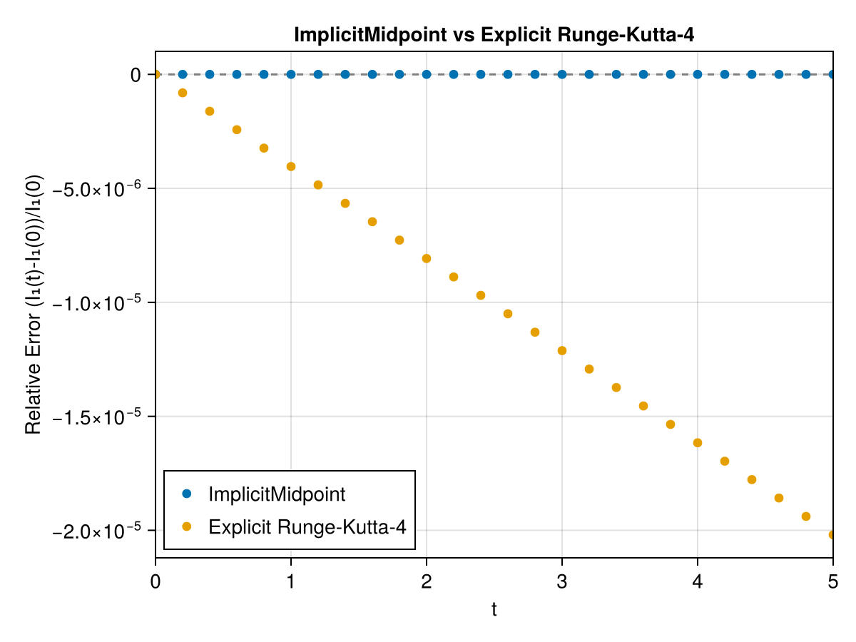

Both symplectic methods (PartitionedGauss and ImplicitMidpoint) conserve the invariant to machine precision, while the non-symplectic RK4 method lets it drift.

Second invariant

The second invariant is the surface integral of the canonical two-form,

\[I_{2} = \int_{S} dq \wedge dp ,\]

the area of the surface $S$. We use a unit square centred at the stable equilibrium.

init2 = (x, y) -> (π + (x - 0.5), y - 0.5)

pi2 = CanonicalSecondPI{Float64, 2}(2_000)

sol2_pg = integrate(PIEnsembleProblem(probh, pi2, init2), PartitionedGauss(1))
sol2_im = integrate(PIEnsembleProblem(probo, pi2, init2), ImplicitMidpoint())
sol2_rk = integrate(PIEnsembleProblem(probo, pi2, init2), RK4())

grid = CanonicalSecondPI{Float64, 2}((15, 15), SecondFinDiffPlan)
solg = integrate(PIEnsembleProblem(probh, grid, init2), PartitionedGauss(1))

plot_surface(grid, solg; xlabel = "q", ylabel = "p")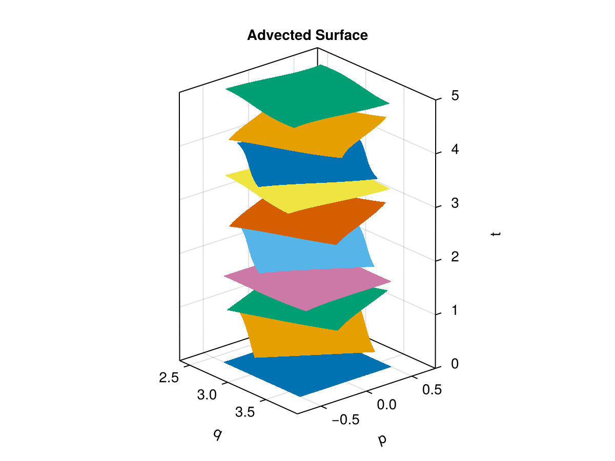

plot_invariant(pi2, sol2_pg; title = "PartitionedGauss")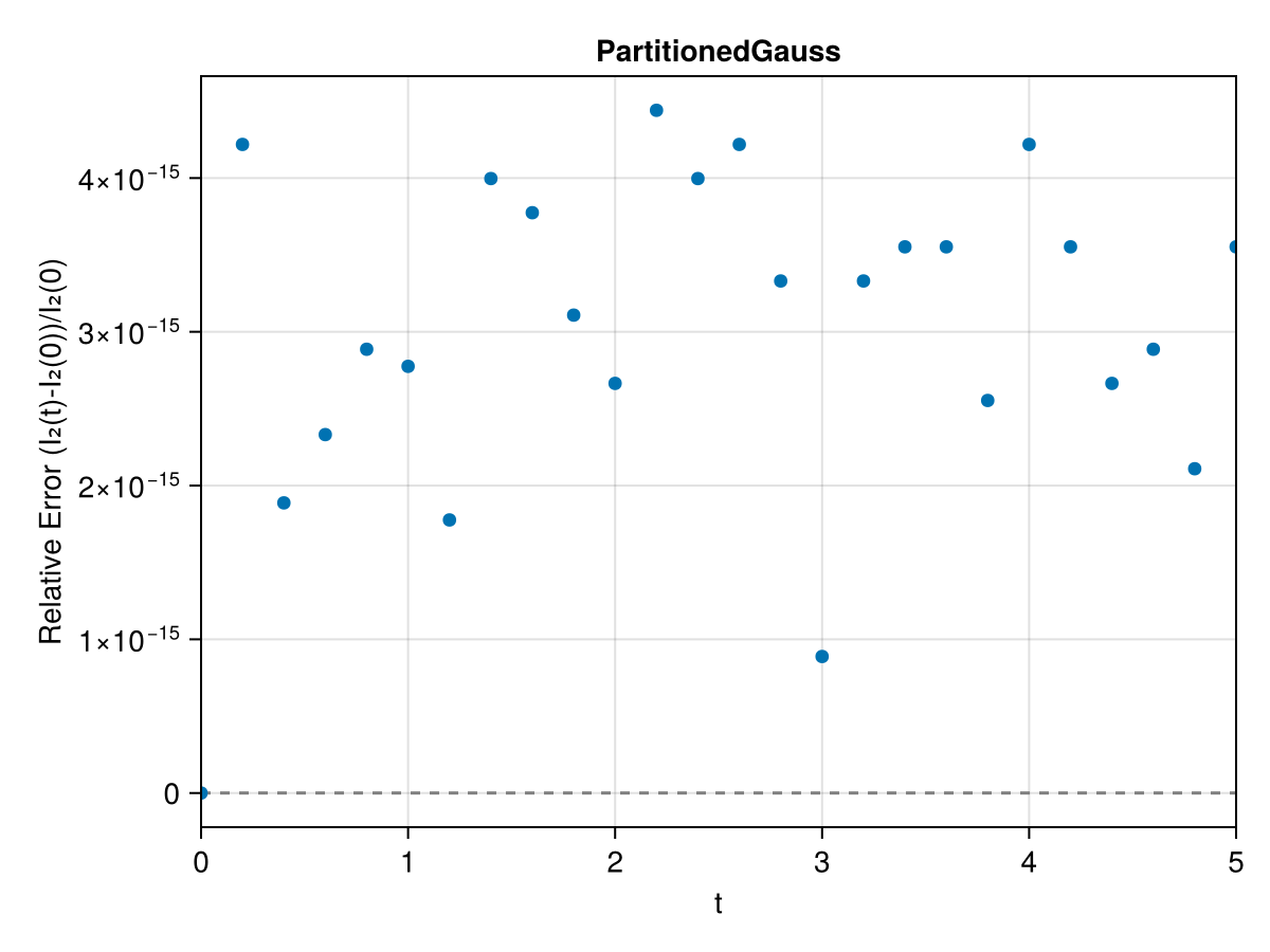

plot_invariant(pi2, "ImplicitMidpoint" => sol2_im, "Explicit Runge-Kutta-4" => sol2_rk;
    title = "ImplicitMidpoint vs Explicit Runge-Kutta-4")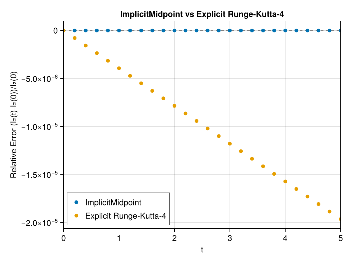

The symplectic methods conserve both invariants even as the curve and surface are distorted by the flow, whereas the non-symplectic explicit Runge-Kutta method lets them drift — exactly the behaviour Poincaré integral invariants are designed to diagnose.