Massless Charged Particle

The massless charged particle in the plane is a noncanonical symplectic system. Its phase space is just the position $x = (x_1, x_2)$, and its dynamics derive from the degenerate Lagrangian

\[L(x, \dot{x}) = A(x) \cdot \dot{x} - \phi(x) ,\]

with magnetic vector potential $A$, electrostatic potential $\phi$ and magnetic field $B(x) = \nabla \times A(x)$. We use the MasslessChargedParticleSingular variant from GeometricProblems.jl, which describes the same physical system in a "singular" magnetic gauge whose vector potential has only one nonzero component,

\[A(x) = - A_0 \, x_2 \, \big( 1 + 2 x_1^2 + \tfrac{2}{3} x_2^2 \big) \begin{pmatrix} 1 \\ 0 \end{pmatrix} , \qquad \phi(x) = E_0 \, \big( \cos x_1 + \sin x_2 \big) , \qquad B(x) = A_0 \, (1 + 2 x_1^2 + 2 x_2^2) .\]

The magnetic field $B$, the electric field and hence the Hamiltonian form of the equations of motion,

\[\dot{x} = \frac{1}{B(x)} \begin{pmatrix} 0 & -1 \\ +1 & 0 \end{pmatrix} \nabla \phi(x) ,\]

are identical to the standard gauge — only the vector potential differs by a gauge transformation. This singular one-form $\vartheta = A(x)$ is exactly the form of the symplectic potential that the DVRK (Degenerate Variational Runge-Kutta) integrator expects, so integrating the degenerate LODEProblem with DVRK preserves the noncanonical symplectic structure $\omega = d\vartheta$ — and with it the Poincaré invariants — to machine accuracy. The plotting functions plot_loop, plot_surface and plot_invariant come from the package's Makie extension, activated by loading CairoMakie.

using PoincareInvariants
using GeometricIntegrators
import GeometricProblems.MasslessChargedParticleSingular as MCP
using StaticArrays
using CairoMakie

prob = MCP.lodeproblem([1.0, 1.0]; timespan = (0.0, 5.0), timestep = 0.1)
par  = parameters(prob)

The invariant forms

The first invariant uses the one-form $\vartheta = A(x)$ (the magnetic vector potential), and the second uses the two-form $\omega = d\vartheta$ (the magnetic field). As in the Lotka-Volterra example, both belong to the LODEProblem itself. PoincareInvariants expects a differential form as an in-place function form(out, t, z, p), which is exactly the convention GeometricProblems uses (ϑ(Θ, t, q, params), ω(Ω, t, q, params)), so we take them from the problem's function tuple with functions(prob) and pass fs.ϑ / fs.ω directly to FirstPI / SecondPI, with no wrapper:

fs = functions(prob)

First invariant

\[I_{1} = \oint_{\gamma} A(x) \cdot dx\]

We advect a small circle of radius $\rho = 0.2$ around the initial position $(1, 1)$ and pass the parameters par to compute! (via plot_invariant) so the form can evaluate $A$.

q₀ = SVector(1.0, 1.0)
ρ  = 0.2

pi1  = FirstPI{Float64, 2}(fs.ϑ, 500)
sol1 = integrate(PIEnsembleProblem(prob, pi1, ϕ -> q₀ .+ ρ .* (cospi(2ϕ), sinpi(2ϕ))), DVRK(Gauss(2)))

The loop is transported and deformed by the flow:

plot_loop(sol1; xlabel = "x₁", ylabel = "x₂")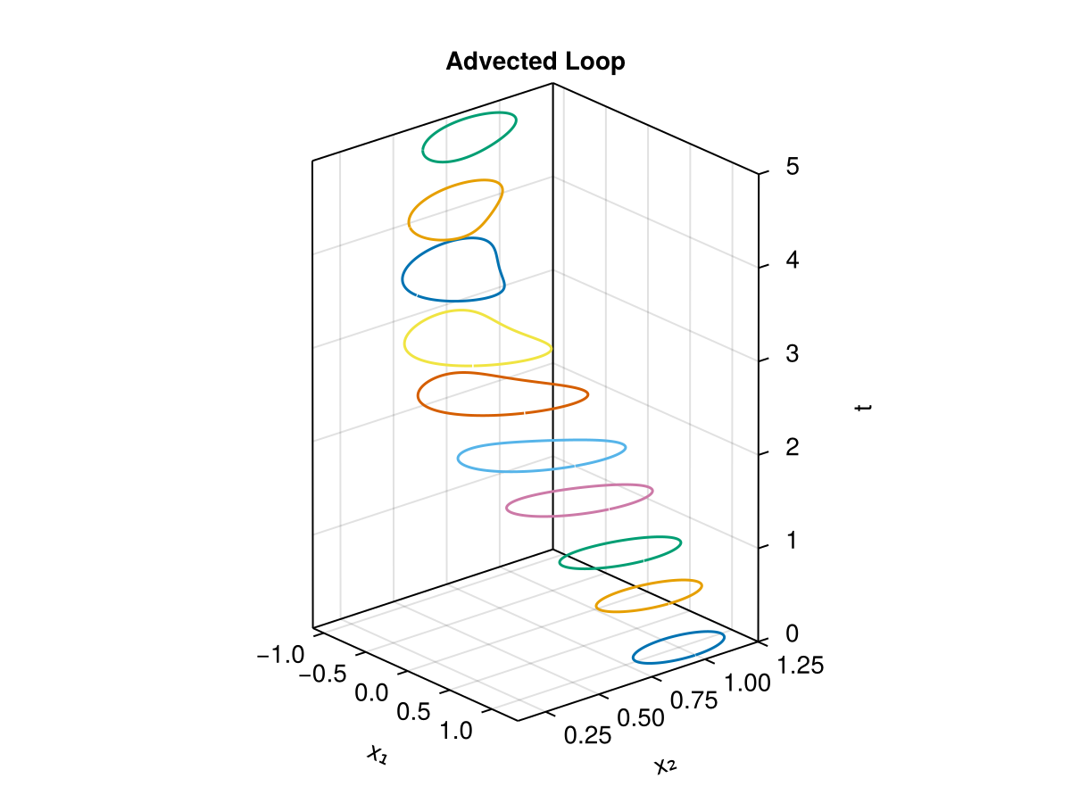

plot_invariant(pi1, sol1; p = par, title = "First Poincaré invariant")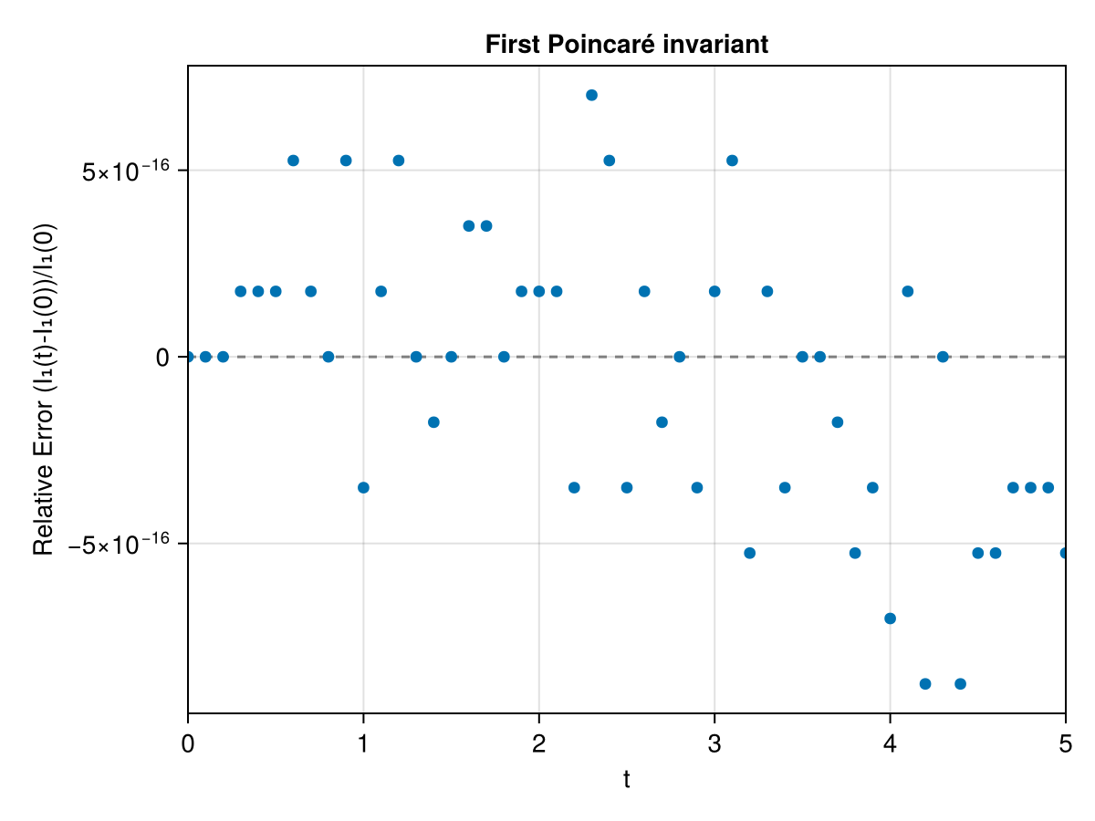

Second invariant

\[I_{2} = \int_{S} \omega = \int_{S} B(x) \, dx_1 \, dx_2\]

is the magnetic flux through the surface $S$. We advect a small square around $(1, 1)$.

pi2  = SecondPI{Float64, 2}(fs.ω, 2_000)
sol2 = integrate(PIEnsembleProblem(prob, pi2, (x, y) -> q₀ .+ ρ .* (2x - 1, 2y - 1)), DVRK(Gauss(2)))

grid = SecondPI{Float64, 2}(fs.ω, (15, 15), SecondFinDiffPlan)
solg = integrate(PIEnsembleProblem(prob, grid, (x, y) -> q₀ .+ ρ .* (2x - 1, 2y - 1)), DVRK(Gauss(2)))

plot_surface(grid, solg; xlabel = "x₁", ylabel = "x₂")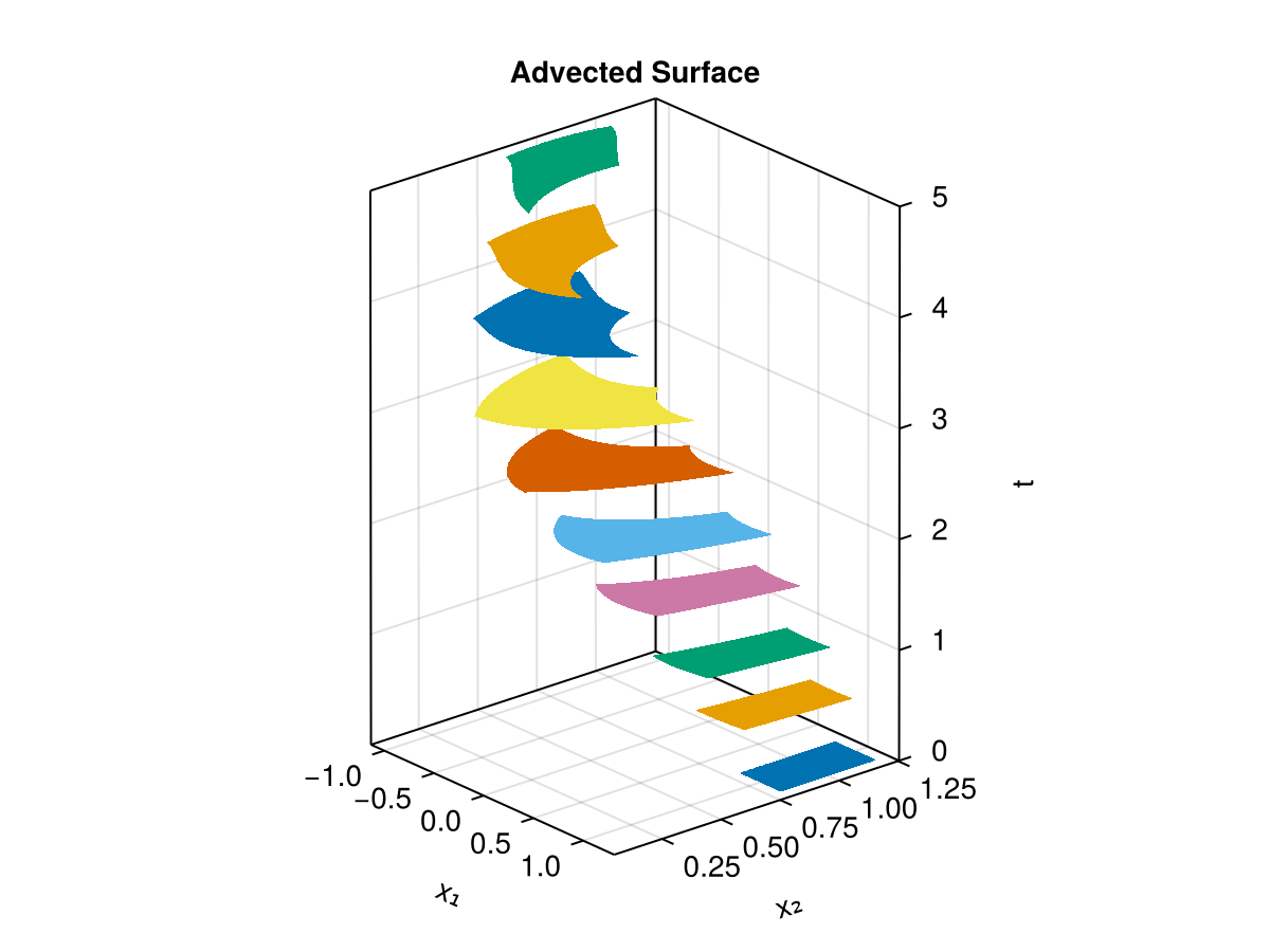

plot_invariant(pi2, sol2; p = par, title = "Second Poincaré invariant")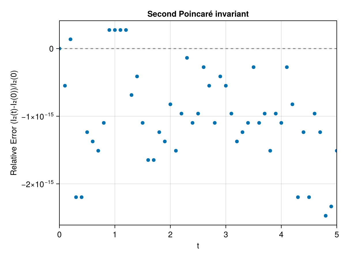

The DVRK(Gauss(2)) method is a fourth-order variational integrator for noncanonical symplectic systems. Because the singular gauge provides exactly the symplectic potential it expects, both invariants are conserved to machine precision as the curve and surface are advected by the flow. A standard, structure-agnostic integrator would let them drift.