Massless Charged Particle

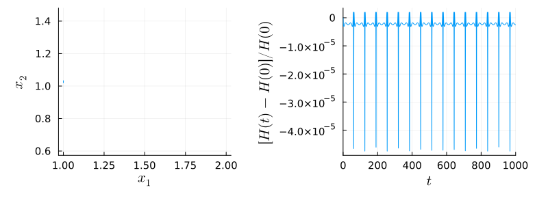
Massless charged particle in 2D

The Lagrangian is given by

\[L(x, \dot{x}) = A(x) \cdot \dot{x} - \phi (x) ,\]

with magnetic vector potential

\[A(x) = \frac{A_0}{2} \big( 1 + x_1^2 + x_2^2 \big) \begin{pmatrix} - x_2 \\ + x_1 \\ \end{pmatrix} ,\]

electrostatic potential

\[\phi(x) = E_0 \, \big( \cos (x_1) + \sin(x_2) \big) ,\]

and magnetic and electric fields

\[\begin{aligned} B(x) &= \nabla \times A(x) = A_0 \, (1 + 2 x_1^2 + 2 x_2^2) , \\ E(x) &= - \nabla \phi(x) = E_0 \, \big( \sin x_1, \, - \cos x_2 \big)^T . \end{aligned}\]

The Hamiltonian form of the equations of motion reads

\[\dot{x} = \frac{1}{B(x)} \begin{pmatrix} \hphantom{-} 0 & - 1 \\ + 1 & \hphantom{+} 0 \\ \end{pmatrix} \nabla \phi (x) .\]

The problem is available in explicit (odeproblem), implicit (iodeproblem, idaeproblem, idaeproblem_spark) and Lagrangian (lodeproblem, ldaeproblem) form. The latter two are built from the Lagrangian $L(x, \dot{x}) = \vartheta (x) \cdot \dot{x} - H(x)$ with one-form $\vartheta = A$ and the symplectic two-form

\[\Omega_{ij} (x) = \frac{\partial \vartheta_i}{\partial x_j} - \frac{\partial \vartheta_j}{\partial x_i} = \begin{pmatrix} \hphantom{+} 0 & - B(x) \\ + B(x) & \hphantom{-} 0 \\ \end{pmatrix} ,\]

so that the Euler-Lagrange equations read $\Omega (x) \, \dot{x} = - \nabla \phi (x)$.

See GeometricProblems.MasslessChargedParticleSingular for a formulation with the same magnetic field but a "singular" (one-component) vector potential, suitable for degenerate variational integrators.

Creates an implicit DAE object for the massless charged particle in 2D.

Creates an implicit DAE object for the massless charged particle in 2D.

Creates an implicit ODE object for the massless charged particle in 2D.

Creates a variational DAE object for the massless charged particle in 2D.

Creates a variational (Lagrangian) ODE object for the massless charged particle in 2D.

Creates an ODE object for the massless charged particle in 2D.

poincare_invariant_1st(N; DT = Float64, plan = PoincareInvariants.DEFAULT_FIRST_PLAN)

Set up the first Poincaré invariant

\[I_1 (t) = \oint_{\gamma_t} \vartheta ,\]

the integral of this module's one-form $\vartheta = A(q)$ over a loop $\gamma_t$, sampled at N points. The Lagrangian is degenerate, so the momentum is not an independent coordinate but determined by $p = \vartheta(q)$, and the loop lives in the two-dimensional configuration space alone.

This is implemented in the MasslessChargedParticlePoincareInvariants extension and becomes available once PoincareInvariants is loaded. Sample a loop with f_loop, advect the sample points with PIEnsembleProblem and evaluate with compute!:

pinv = poincare_invariant_1st(200)
prob = iodeproblem(; timespan = (0.0, 1E2), timestep = 1E-1)
sol  = integrate(PIEnsembleProblem(prob, pinv, f_loop), VPRKGauss(2))
I₁   = compute!(pinv, sol, parameters(prob))

Note that I₁ is preserved by a variational integrator only to the order of the discretisation, not exactly: the numerical solution satisfies $p = \vartheta(q)$ only up to the truncation error.

The two gauges of the massless charged particle differ by a gauge transformation, which changes $\vartheta$ by an exact form. Since the integral of an exact form over a closed loop vanishes, both give the same $I_1$ for the same loop.

See also poincare_invariant_2nd.

poincare_invariant_2nd(N; DT = Float64, plan = PoincareInvariants.DEFAULT_SECOND_PLAN)

Set up the second Poincaré invariant

\[I_2 (t) = \int_{\sigma_t} \omega ,\]

the integral of this module's two-form $\omega$, whose only component is $\omega_{12} = -B(q)$, over a surface $\sigma_t$ sampled at N points. As for the first invariant the surface lives in the two-dimensional configuration space alone. The default plan samples at Padua points and rounds N up to the next Padua number, so the invariant may use slightly more points than requested; getpointnum reports how many.

This is implemented in the MasslessChargedParticlePoincareInvariants extension and becomes available once PoincareInvariants is loaded. It is used exactly like the first invariant, with f_surface in place of f_loop. If the surface is the region a loop bounds, then $I_2$ over the surface and $I_1$ over the loop agree by Stokes' theorem — f_surface is not that region for f_loop, but lies inside it.

Unlike $\vartheta$, $\omega = -d\vartheta$ is gauge invariant, so both gauges of the massless charged particle share the same two-form.

See also poincare_invariant_1st.

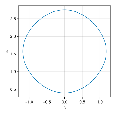
Massless charged particle in 2D with "singular" vector potential

The Lagrangian is given by

\[L(x, \dot{x}) = A(x) \cdot \dot{x} - \phi (x) ,\]

with the "singular" (one-component) magnetic vector potential

\[A(x) = - A_0 \, x_2 \, \big( 1 + 2 x_1^2 + \tfrac{2}{3} x_2^2 \big) \begin{pmatrix} 1 \\ 0 \\ \end{pmatrix} ,\]

electrostatic potential

\[\phi(x) = E_0 \, \big( \cos (x_1) + \sin(x_2) \big) ,\]

and magnetic and electric fields

\[\begin{aligned} B(x) &= \nabla \times A(x) = A_0 \, (1 + 2 x_1^2 + 2 x_2^2) , \\ E(x) &= - \nabla \phi(x) = E_0 \, \big( \sin x_1, \, - \cos x_2 \big)^T . \end{aligned}\]

The Hamiltonian form of the equations of motion reads

\[\dot{x} = \frac{1}{B(x)} \begin{pmatrix} \hphantom{-} 0 & - 1 \\ + 1 & \hphantom{+} 0 \\ \end{pmatrix} \nabla \phi (x) .\]

This is the same physical system as GeometricProblems.MasslessChargedParticle: the magnetic field $B$, electric field $E$ and hence the dynamics are identical. Only the vector potential differs by a gauge transformation, chosen here so that its second component vanishes ($A_2 = 0$). This "singular" one-form yields the same Euler-Lagrange equations but a different variational integrator, and is the form required by the degenerate variational integrator (DVI) method of GeometricIntegrators.

The problem is available in explicit (odeproblem), implicit (iodeproblem, idaeproblem, idaeproblem_spark) and Lagrangian (lodeproblem, ldaeproblem) form. The latter two are built from the Lagrangian $L(x, \dot{x}) = \vartheta (x) \cdot \dot{x} - H(x)$ with one-form $\vartheta = A$ and the symplectic two-form

\[\Omega_{ij} (x) = \frac{\partial \vartheta_i}{\partial x_j} - \frac{\partial \vartheta_j}{\partial x_i} = \begin{pmatrix} \hphantom{+} 0 & - B(x) \\ + B(x) & \hphantom{-} 0 \\ \end{pmatrix} ,\]

so that the Euler-Lagrange equations read $\Omega (x) \, \dot{x} = - \nabla \phi (x)$. Since the gauge transformation shifts $\vartheta$ only by an exact one-form, $\Omega$ is the same as for GeometricProblems.MasslessChargedParticle, while the Lagrangian differs.

Creates an implicit DAE object for the massless charged particle in 2D.

Creates an implicit DAE object for the massless charged particle in 2D.

Creates an implicit ODE object for the massless charged particle in 2D.

Creates a variational DAE object for the massless charged particle in 2D.

Creates a variational (Lagrangian) ODE object for the massless charged particle in 2D.

Creates an ODE object for the massless charged particle in 2D.

poincare_invariant_1st(N; DT = Float64, plan = PoincareInvariants.DEFAULT_FIRST_PLAN)

Set up the first Poincaré invariant

\[I_1 (t) = \oint_{\gamma_t} \vartheta ,\]

the integral of this module's one-form $\vartheta = A(q)$ over a loop $\gamma_t$, sampled at N points. The Lagrangian is degenerate, so the momentum is not an independent coordinate but determined by $p = \vartheta(q)$, and the loop lives in the two-dimensional configuration space alone.

This is implemented in the MasslessChargedParticlePoincareInvariants extension and becomes available once PoincareInvariants is loaded. Sample a loop with f_loop, advect the sample points with PIEnsembleProblem and evaluate with compute!:

pinv = poincare_invariant_1st(200)
prob = iodeproblem(; timespan = (0.0, 1E2), timestep = 1E-1)
sol  = integrate(PIEnsembleProblem(prob, pinv, f_loop), VPRKGauss(2))
I₁   = compute!(pinv, sol, parameters(prob))

Note that I₁ is preserved by a variational integrator only to the order of the discretisation, not exactly: the numerical solution satisfies $p = \vartheta(q)$ only up to the truncation error.

The two gauges of the massless charged particle differ by a gauge transformation, which changes $\vartheta$ by an exact form. Since the integral of an exact form over a closed loop vanishes, both give the same $I_1$ for the same loop.

See also poincare_invariant_2nd.

poincare_invariant_2nd(N; DT = Float64, plan = PoincareInvariants.DEFAULT_SECOND_PLAN)

Set up the second Poincaré invariant

\[I_2 (t) = \int_{\sigma_t} \omega ,\]

the integral of this module's two-form $\omega$, whose only component is $\omega_{12} = -B(q)$, over a surface $\sigma_t$ sampled at N points. As for the first invariant the surface lives in the two-dimensional configuration space alone. The default plan samples at Padua points and rounds N up to the next Padua number, so the invariant may use slightly more points than requested; getpointnum reports how many.

This is implemented in the MasslessChargedParticlePoincareInvariants extension and becomes available once PoincareInvariants is loaded. It is used exactly like the first invariant, with f_surface in place of f_loop. If the surface is the region a loop bounds, then $I_2$ over the surface and $I_1$ over the loop agree by Stokes' theorem — f_surface is not that region for f_loop, but lies inside it.

Unlike $\vartheta$, $\omega = -d\vartheta$ is gauge invariant, so both gauges of the massless charged particle share the same two-form.

See also poincare_invariant_1st.