Lotka-Volterra 2d
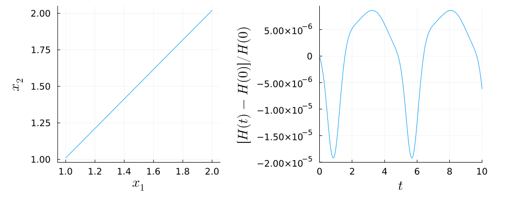
Lotka–Volterra models are used in mathematical biology for modelling population dynamics of animal species, as well as many other fields where predator-prey and similar models appear. The dynamics of the growth of two interacting species can be modelled by the following noncanonical Hamiltonian system
\[\dot{q} = \begin{pmatrix} \hphantom{-} 0 & + q_1 q_2 \\ - q_1 q_2 & \hphantom{+} 0 \\ \end{pmatrix} \nabla H (q) , \quad H (q) = a_1 \, q_1 + a_2 \, q_2 + b_1 \, \log q_1 + b_2 \, \log q_2 .\]
Sub-models
The Euler-Lagrange equations of the Lotka-Volterra model can be obtained from different Lagrangians, which are connected by gauge transformations. Although they all lead to the same equations of motion, they lead to different variational integrators. Therefore different models based on different Lagrangians are implemented.
GeometricProblems.LotkaVolterra2d — Module
Lotka-Volterra model in 2D
\[\begin{aligned} L (q, \dot{q}) &= \bigg( q_2 + \frac{\log q_2}{q_1} \bigg) \, \dot{q_1} + q_1 \, \dot{q_2} - H(q) , \\ H(q) &= a_1 \, q_1 + a_2 \, q_2 + b_1 \, \log q_1 + b_2 \, \log q_2 \end{aligned}\]
GeometricProblems.LotkaVolterra2dSymmetric — Module
Lotka-Volterra model in 2D with symmetric Lagrangian
\[\begin{aligned} L (q, \dot{q}) &= \frac{1}{2} \frac{\log q_2}{q_1} \, \dot{q_1} - \frac{1}{2} \frac{\log q_1}{q_2} \, \dot{q_2} - H(q) , \\ H(q) &= a_1 \, q_1 + a_2 \, q_2 + b_1 \, \log q_1 + b_2 \, \log q_2 \end{aligned}\]
This Lagrangian is a slight generalization of Equation (5) in José Fernández-Núñez, Lagrangian Structure of the Two-Dimensional Lotka-Volterra System, International Journal of Theoretical Physics, Vol. 37, No. 9, pp. 2457-2462, 1998.
GeometricProblems.LotkaVolterra2dSingular — Module
Lotka-Volterra model in 2D with "singular" Lagrangian
\[\begin{aligned} L (q, \dot{q}) &= \frac{\log q_2}{q_1} \, \dot{q_1} - H(q) , \\ H(q) &= a_1 \, q_1 + a_2 \, q_2 + b_1 \, \log q_1 + b_2 \, \log q_2 \end{aligned}\]
This Lagrangian is equivalent to the Lagrangian of the symmetric Lotka-Volterra model. It differs only by a gauge transformation with the term $- 1/2 \, d(\log(q_1) \log(q_2))/dt$. It leads to the same Euler-Lagrange equations but to a different variational integrator.
GeometricProblems.LotkaVolterra2dGauge — Module
Lotka-Volterra model in 2D with symmetric Lagrangian with gauge term
\[\begin{aligned} L (q, \dot{q}) &= \bigg( q_2 + \frac{1}{2} \frac{\log q_2}{q_1} \bigg) \, \dot{q_1} + \bigg( q_1 - \frac{1}{2} \frac{\log q_1}{q_2} \bigg) \, \dot{q_2} - H(q) , \\ H(q) &= a_1 \, q_1 + a_2 \, q_2 + b_1 \, \log q_1 + b_2 \, \log q_2 \end{aligned}\]
This Lagrangian is equivalent to the Lagrangian of the symmetric Lotka-Volterra model. It differs only by a gauge transformation with the term $d(q_1 q_2)/dt$. It leads to the same Euler-Lagrange equations but to a different variational integrator.
User Functions
The plotting functions (plot_solution, plot_phase_portrait, plot_traces) are provided by the LotkaVolterra2dPlots extension and become available once a Makie backend such as CairoMakie is loaded.
GeometricProblems.LotkaVolterra2d.daeproblem — Function
Creates a DAE object for the Lotka-Volterra 2D model.
GeometricProblems.LotkaVolterra2d.hdaeproblem — Function
Creates a Hamiltonian DAE object for the Lotka-Volterra 2D model.
GeometricProblems.LotkaVolterra2d.hodeproblem — Function
Creates a Hamiltonian ODE object for the Lotka-Volterra 2D model.
GeometricProblems.LotkaVolterra2d.idaeproblem — Function
Creates an implicit DAE object for the Lotka-Volterra 2D model.
GeometricProblems.LotkaVolterra2d.idaeproblem_spark — Function
Creates an implicit DAE object for the Lotka-Volterra 2D model.
GeometricProblems.LotkaVolterra2d.iodeproblem — Function
Creates an implicit ODE object for the Lotka-Volterra 2D model.
GeometricProblems.LotkaVolterra2d.iodeproblem_dg — Function
Creates an implicit ODE object for the Lotka-Volterra 2D model for use with DG integrators.
GeometricProblems.LotkaVolterra2d.ldaeproblem — Function
Creates a variational DAE object for the Lotka-Volterra 2D model.
GeometricProblems.LotkaVolterra2d.ldaeproblem_slrk — Function
Creates a variational DAE object for the Lotka-Volterra 2D model for use with SLRK integrators.
GeometricProblems.LotkaVolterra2d.lodeproblem — Function
Creates a variational ODE object for the Lotka-Volterra 2D model.
GeometricProblems.LotkaVolterra2d.odeproblem — Function
Creates an ODE object for the Lotka-Volterra 2D model.
GeometricProblems.LotkaVolterra2d.pdaeproblem — Function
Creates a partitioned DAE object for the Lotka-Volterra 2D model.
GeometricProblems.LotkaVolterra2d.podeproblem — Function
Creates a partitioned ODE object for the Lotka-Volterra 2D model.
GeometricProblems.LotkaVolterra2d.poincare_invariant_1st — Function
poincare_invariant_1st(N; DT = Float64, plan = PoincareInvariants.DEFAULT_FIRST_PLAN)Set up the first Poincaré invariant
\[I_1 (t) = \oint_{\gamma_t} \vartheta ,\]
the integral of this module's one-form $\vartheta$ over a loop $\gamma_t$, sampled at N points. The Lagrangian is degenerate, so the momentum is not an independent coordinate but determined by $p = \vartheta(q)$, and the loop lives in the two-dimensional configuration space alone.
This is implemented in the LotkaVolterra2dPoincareInvariants extension and becomes available once PoincareInvariants is loaded. Sample a loop with f_loop, advect the sample points with PIEnsembleProblem and evaluate with compute!:
pinv = poincare_invariant_1st(200)
prob = iodeproblem(; timespan = (0.0, 1E2), timestep = 1E-1)
sol  = integrate(PIEnsembleProblem(prob, pinv, f_loop), VPRKGauss(2))
I₁   = compute!(pinv, sol, parameters(prob))
Note that I₁ is preserved by a variational integrator only to the order of the discretisation, not exactly: the numerical solution satisfies $p = \vartheta(q)$ only up to the truncation error.
The four gauges of the Lotka-Volterra 2d model differ by gauge transformations, which change $\vartheta$ by an exact form. Since the integral of an exact form over a closed loop vanishes, all four give the same $I_1$ for the same loop.
See also poincare_invariant_2nd.
GeometricProblems.LotkaVolterra2d.poincare_invariant_2nd — Function
poincare_invariant_2nd(N; DT = Float64, plan = PoincareInvariants.DEFAULT_SECOND_PLAN)Set up the second Poincaré invariant
\[I_2 (t) = \int_{\sigma_t} \omega ,\]
the integral of this module's two-form $\omega$ over a surface $\sigma_t$, sampled at N points. As for the first invariant the surface lives in the two-dimensional configuration space alone. The default plan samples at Padua points and rounds N up to the next Padua number, so the invariant may use slightly more points than requested; getpointnum reports how many.
This is implemented in the LotkaVolterra2dPoincareInvariants extension and becomes available once PoincareInvariants is loaded. It is used exactly like the first invariant, with f_surface in place of f_loop. If the surface is the region a loop bounds, then $I_2$ over the surface and $I_1$ over the loop agree by Stokes' theorem — f_surface is not that region for f_loop, but lies inside it.
Unlike $\vartheta$, $\omega = -d\vartheta$ is gauge invariant, so all four gauges of the Lotka-Volterra 2d model share the same two-form.
See also poincare_invariant_1st.
Poincaré invariants
The Poincaré invariants are provided by the LotkaVolterra2dPoincareInvariants extension and become available once PoincareInvariants is loaded. Each of the four sub-models carries its own pair, built over its own one- and two-form. The pair belonging to LotkaVolterra2d is listed under User Functions above.
GeometricProblems.LotkaVolterra2dSymmetric.poincare_invariant_1st — Function
poincare_invariant_1st(N; DT = Float64, plan = PoincareInvariants.DEFAULT_FIRST_PLAN)Set up the first Poincaré invariant
\[I_1 (t) = \oint_{\gamma_t} \vartheta ,\]
the integral of this module's one-form $\vartheta$ over a loop $\gamma_t$, sampled at N points. The Lagrangian is degenerate, so the momentum is not an independent coordinate but determined by $p = \vartheta(q)$, and the loop lives in the two-dimensional configuration space alone.
This is implemented in the LotkaVolterra2dPoincareInvariants extension and becomes available once PoincareInvariants is loaded. Sample a loop with f_loop, advect the sample points with PIEnsembleProblem and evaluate with compute!:
pinv = poincare_invariant_1st(200)
prob = iodeproblem(; timespan = (0.0, 1E2), timestep = 1E-1)
sol  = integrate(PIEnsembleProblem(prob, pinv, f_loop), VPRKGauss(2))
I₁   = compute!(pinv, sol, parameters(prob))
Note that I₁ is preserved by a variational integrator only to the order of the discretisation, not exactly: the numerical solution satisfies $p = \vartheta(q)$ only up to the truncation error.
The four gauges of the Lotka-Volterra 2d model differ by gauge transformations, which change $\vartheta$ by an exact form. Since the integral of an exact form over a closed loop vanishes, all four give the same $I_1$ for the same loop.
See also poincare_invariant_2nd.
GeometricProblems.LotkaVolterra2dSymmetric.poincare_invariant_2nd — Function
poincare_invariant_2nd(N; DT = Float64, plan = PoincareInvariants.DEFAULT_SECOND_PLAN)Set up the second Poincaré invariant
\[I_2 (t) = \int_{\sigma_t} \omega ,\]
the integral of this module's two-form $\omega$ over a surface $\sigma_t$, sampled at N points. As for the first invariant the surface lives in the two-dimensional configuration space alone. The default plan samples at Padua points and rounds N up to the next Padua number, so the invariant may use slightly more points than requested; getpointnum reports how many.
This is implemented in the LotkaVolterra2dPoincareInvariants extension and becomes available once PoincareInvariants is loaded. It is used exactly like the first invariant, with f_surface in place of f_loop. If the surface is the region a loop bounds, then $I_2$ over the surface and $I_1$ over the loop agree by Stokes' theorem — f_surface is not that region for f_loop, but lies inside it.
Unlike $\vartheta$, $\omega = -d\vartheta$ is gauge invariant, so all four gauges of the Lotka-Volterra 2d model share the same two-form.
See also poincare_invariant_1st.
GeometricProblems.LotkaVolterra2dSingular.poincare_invariant_1st — Function
poincare_invariant_1st(N; DT = Float64, plan = PoincareInvariants.DEFAULT_FIRST_PLAN)Set up the first Poincaré invariant
\[I_1 (t) = \oint_{\gamma_t} \vartheta ,\]
the integral of this module's one-form $\vartheta$ over a loop $\gamma_t$, sampled at N points. The Lagrangian is degenerate, so the momentum is not an independent coordinate but determined by $p = \vartheta(q)$, and the loop lives in the two-dimensional configuration space alone.
This is implemented in the LotkaVolterra2dPoincareInvariants extension and becomes available once PoincareInvariants is loaded. Sample a loop with f_loop, advect the sample points with PIEnsembleProblem and evaluate with compute!:
pinv = poincare_invariant_1st(200)
prob = iodeproblem(; timespan = (0.0, 1E2), timestep = 1E-1)
sol  = integrate(PIEnsembleProblem(prob, pinv, f_loop), VPRKGauss(2))
I₁   = compute!(pinv, sol, parameters(prob))
Note that I₁ is preserved by a variational integrator only to the order of the discretisation, not exactly: the numerical solution satisfies $p = \vartheta(q)$ only up to the truncation error.
The four gauges of the Lotka-Volterra 2d model differ by gauge transformations, which change $\vartheta$ by an exact form. Since the integral of an exact form over a closed loop vanishes, all four give the same $I_1$ for the same loop.
See also poincare_invariant_2nd.
GeometricProblems.LotkaVolterra2dSingular.poincare_invariant_2nd — Function
poincare_invariant_2nd(N; DT = Float64, plan = PoincareInvariants.DEFAULT_SECOND_PLAN)Set up the second Poincaré invariant
\[I_2 (t) = \int_{\sigma_t} \omega ,\]
the integral of this module's two-form $\omega$ over a surface $\sigma_t$, sampled at N points. As for the first invariant the surface lives in the two-dimensional configuration space alone. The default plan samples at Padua points and rounds N up to the next Padua number, so the invariant may use slightly more points than requested; getpointnum reports how many.
This is implemented in the LotkaVolterra2dPoincareInvariants extension and becomes available once PoincareInvariants is loaded. It is used exactly like the first invariant, with f_surface in place of f_loop. If the surface is the region a loop bounds, then $I_2$ over the surface and $I_1$ over the loop agree by Stokes' theorem — f_surface is not that region for f_loop, but lies inside it.
Unlike $\vartheta$, $\omega = -d\vartheta$ is gauge invariant, so all four gauges of the Lotka-Volterra 2d model share the same two-form.
See also poincare_invariant_1st.
GeometricProblems.LotkaVolterra2dGauge.poincare_invariant_1st — Function
poincare_invariant_1st(N; DT = Float64, plan = PoincareInvariants.DEFAULT_FIRST_PLAN)Set up the first Poincaré invariant
\[I_1 (t) = \oint_{\gamma_t} \vartheta ,\]
the integral of this module's one-form $\vartheta$ over a loop $\gamma_t$, sampled at N points. The Lagrangian is degenerate, so the momentum is not an independent coordinate but determined by $p = \vartheta(q)$, and the loop lives in the two-dimensional configuration space alone.
This is implemented in the LotkaVolterra2dPoincareInvariants extension and becomes available once PoincareInvariants is loaded. Sample a loop with f_loop, advect the sample points with PIEnsembleProblem and evaluate with compute!:
pinv = poincare_invariant_1st(200)
prob = iodeproblem(; timespan = (0.0, 1E2), timestep = 1E-1)
sol  = integrate(PIEnsembleProblem(prob, pinv, f_loop), VPRKGauss(2))
I₁   = compute!(pinv, sol, parameters(prob))
Note that I₁ is preserved by a variational integrator only to the order of the discretisation, not exactly: the numerical solution satisfies $p = \vartheta(q)$ only up to the truncation error.
The four gauges of the Lotka-Volterra 2d model differ by gauge transformations, which change $\vartheta$ by an exact form. Since the integral of an exact form over a closed loop vanishes, all four give the same $I_1$ for the same loop.
See also poincare_invariant_2nd.
GeometricProblems.LotkaVolterra2dGauge.poincare_invariant_2nd — Function
poincare_invariant_2nd(N; DT = Float64, plan = PoincareInvariants.DEFAULT_SECOND_PLAN)Set up the second Poincaré invariant
\[I_2 (t) = \int_{\sigma_t} \omega ,\]
the integral of this module's two-form $\omega$ over a surface $\sigma_t$, sampled at N points. As for the first invariant the surface lives in the two-dimensional configuration space alone. The default plan samples at Padua points and rounds N up to the next Padua number, so the invariant may use slightly more points than requested; getpointnum reports how many.
This is implemented in the LotkaVolterra2dPoincareInvariants extension and becomes available once PoincareInvariants is loaded. It is used exactly like the first invariant, with f_surface in place of f_loop. If the surface is the region a loop bounds, then $I_2$ over the surface and $I_1$ over the loop agree by Stokes' theorem — f_surface is not that region for f_loop, but lies inside it.
Unlike $\vartheta$, $\omega = -d\vartheta$ is gauge invariant, so all four gauges of the Lotka-Volterra 2d model share the same two-form.
See also poincare_invariant_1st.