Variational Partitioned Runge-Kutta Integrators
Variational partitioned Runge-Kutta methods solve Lagrangian systems in implicit form, i.e.,
\[\begin{aligned} p &= \dfrac{\partial L}{\partial \dot{q}} (q, \dot{q}) , & \dot{p} &= \dfrac{\partial L}{\partial q} (q, \dot{q}) , \end{aligned}\]
by the following scheme,
\[\begin{equation}\label{eq:vprk} \begin{aligned} P_{n,i} &= \dfrac{\partial L}{\partial v} (Q_{n,i}, V_{n,i}) , & Q_{n,i} &= q_{n} + h \sum \limits_{j=1}^{s} a_{ij} \, V_{n,j} , & q_{n+1} &= q_{n} + h \sum \limits_{i=1}^{s} b_{i} \, V_{n,i} , \\ F_{k,i} &= \dfrac{\partial L}{\partial q} (Q_{n,i}, V_{n,i}) , & P_{n,j} &= p_{n} + h \sum \limits_{i=1}^{s} \bar{a}_{ij} \, F_{n,j} , & p_{n+1} &= p_{n} + h \sum \limits_{i=1}^{s} b_{i} \, F_{n,i} . \end{aligned} \end{equation}\]
Here, $s$ denotes the number of internal stages, $a_{ij}$ and $\bar{a}_{ij}$ are the coefficients of the Runge-Kutta method and $b_{i}$ and $\bar{b}_{i}$ the corresponding weights. If the coefficients satisfy the symplecticity conditions,
\[\begin{aligned} b_{i} \bar{a}_{ij} + \bar{b}_{j} a_{ji} &= b_{i} \bar{b}_{j} & & \text{and} & \bar{b}_{i} &= b_{i} , \end{aligned}\]
these methods correspond to the position-momentum form of the discrete Lagrangian [[9]]
\[\begin{equation}\label{eq:vprk-discrete-lagrangian} L_{d} (q_{n}, q_{n+1}) = h \sum \limits_{i=1}^{s} b_{i} \, L \big( Q_{n,i}, V_{n,i} \big) . \end{equation}\]
While these integrators show favourable properties for systems with regular Lagrangian, they are usually not applicable for degenerate Lagrangian systems, in particular those with Lagrangians of the form $L (q, \dot{q}) = \vartheta(q) \cdot \dot{q} - H(q)$. While variational integrators are still applicable in the case of $\vartheta$ being a linear function of $q$, they are often found to be unstable when $\vartheta$ is a nonlinear function of $q$ as is the case with Lotka-Volterra systems, various nonlinear oscillators, guiding centre dynamics and other reduced charged particle models. To mitigate this problem, projection methods have been developed, which can be used in conjunction with variational integrators. These projected variational integrators provide long-time stable methods for general degenerate Lagrangian systems that maintain conservation of energy and momenta over long integration periods [[14]].
GeometricIntegrators.jl provides the following VPRK methods:
| Integrator | Description |
|---|---|
VPRK | Variational Partitioned Runge-Kutta (VPRK) integrator without projection |
VPRKpStandard | VPRK integrator with standard projection |
VPRKpSymmetric | VPRK integrator with symmetric projection |
VPRKpMidpoint | VPRK integrator with midpoint projection |
VPRKpVariational | VPRK integrator with variational projection (unstable) |
VPRKpSecondary | VPRK integrator with projection on secondary constraint |
VPRKpInternal | Gauss-Legendre VPRK integrator with projection on internal stages of Runge-Kutta method |
For testing purposes VPRKpStandard provides some additional constructors (note that these methods are generally unstable):
| Integrator | Description |
|---|---|
VPRKpVariationalQ | VPRK integrator with variational projection on $(q_{n}, p_{n+1})$ |
VPRKpVariationalP | VPRK integrator with variational projection on $(p_{n}, q_{n+1})$ |
VPRKpSymplectic | VPRK integrator with symplectic projection |
All of the above integrators are applied to either an IODEProblem or LODEProblem and instantiated as follows:
int = GeometricIntegrator(iode, VPRK(Gauss(1)))where the constructor of each method needs to be supplied with a Runge-Kutta or partitioned Runge-Kutta method. The only exception is VPRKpSecondary which can only be applied to an LODEProblem as it needs some additional functions which are only defined for variational problems.
Discrete Action Princtiple
Symplectic partitioned Runge-Kutta integrators have been shown to be variational integrators [[9], [5]]. Here, the discrete Lagrangian \eqref{eq:vprk-discrete-lagrangian} has $s$ internal points (or stages) located at $t_{n} + h c_{i}$ with weights $b_{i}$ which are all non-zero and sum up to one. The internal stages $Q_{n,i} \approx q(t_{n} + h c_{i})$ are given by
\[Q_{n,i} = q_{n} + h \sum \limits_{j=1}^{s} a_{ij} \, V_{n,j} .\]
In contrast to the composition methods, we do not require $c_{1} = 0$ and $c_{s} = 1$. Instead the discrete action is extremised under the constraints
\[q_{n+1} = q_{n} + h \sum \limits_{i=1}^{s} b_{i} \, V_{n,i} ,\]
which we add to the action with the Lagrange multiplier $\lambda_{n+1}$, so that we can write
\[\begin{equation}\label{eq:vprk-action-gauss} \mathcal{A}_{d} = \sum \limits_{n=1}^{N-1} \bigg[ h \sum \limits_{i=1}^{s} b_{i} \, L \big( Q_{n,i}, V_{n,1} \big) + \lambda_{n+1} \cdot \bigg( q_{n+1} - q_{n} - h \sum \limits_{i=1}^{s} b_{i} \, V_{n,i} \bigg) \bigg] . \end{equation}\]
Computing variations of the action leads to
\[\begin{aligned} \delta \mathcal{A}_{d} &= \sum \limits_{n=1}^{N-1}\left[ h \sum \limits_{i=1}^{s} h b_{i} a_{ij} \, \dfrac{\partial L}{\partial q} (Q_{n,i}, V_{n,i}) + h b_{j} \, \dfrac{\partial L}{\partial v} (Q_{n,j}, V_{n,j}) - h b_{j} \, \lambda_{n+1} \right] \cdot \delta V_{n,j} \\ &+ \sum \limits_{n=1}^{N-1}\left[ h \sum \limits_{i=1}^{s} b_{i} \, \dfrac{\partial L}{\partial q} (Q_{n,i}, V_{n,i}) - \lambda_{n+1} + \lambda_{n} \right] \cdot \delta q_{n} \\ &+ \sum \limits_{n=1}^{N-1} \bigg[ q_{n+1} - q_{n} - h \sum \limits_{i=1}^{s} b_{i} \, V_{n,i} \bigg] \cdot \delta \lambda_{n+1} = 0 . \end{aligned}\]
We define discrete forces and momenta as
\[F_{n,i} = \dfrac{\partial L}{\partial q} (Q_{n,i}, V_{n,i}) \hspace{3em} \text{and} \hspace{3em} P_{n,i} = \dfrac{\partial L}{\partial v} (Q_{n,i}, V_{n,i}) ,\]
so that the terms of the variation which are multiplying $\delta V_{n,j}$ become
\[P_{n,j} = \lambda_{n+1} - h \sum \limits_{i=1}^{s} \dfrac{b_{i} a_{ij}}{b_{j}} \, F_{n,i} .\]
The terms of the variations which are multiplying $\delta q_{n}$ become
\[\lambda_{n+1} = \lambda_{n} + h \sum \limits_{i=1}^{s} b_{i} \, F_{n,i} .\]
Similar to classical variational integrators, we can use the discrete fibre derivative
\[\begin{equation}\label{eq:discrete-fibre-derivative} \begin{aligned} \mathbb{F}^{-} L_{d} : (q_{n}, q_{n+1}) &\mapsto (q_{n}, p_{n}) = \big( q_{n} , - D_{1} L_{d} (q_{n}, q_{n+1}) \big) , \\ \mathbb{F}^{+} L_{d} : (q_{n}, q_{n+1}) &\mapsto (q_{n+1}, p_{n+1}) = \big( q_{n+1}, D_{2} L_{d} (q_{n}, q_{n+1}) \big) . \end{aligned} \end{equation}\]
to define the position-momentum form of the integrator,
\[\begin{equation}\label{eq:vi-position-momentum-form} \begin{aligned} p_{n } &= - D_{1} L_{d} (q_{n}, q_{n+1}) = \lambda_{n+1} - h \sum \limits_{i=1}^{s} b_{i} \, F_{n,i} , \\ p_{n+1} &= \hphantom{-} D_{2} L_{d} (q_{n}, q_{n+1}) = \lambda_{n+1} . \end{aligned} \end{equation}\]
Replacing $\lambda_{n+1}$ in the second equation with its expression obtained from the first equation, we get
\[p_{n+1} = p_{n} + h \sum \limits_{i=1}^{s} v_{i} \, F_{n,i} ,\]
which states that the second symplecticity condition ($b_{i} = \bar{b}_{i}$) is automatically satisfied. In the same fashion, we obtain
\[P_{n,j} = p_{n} + h \sum \limits_{i=1}^{s} \bar{a}_{ij} \, F_{n,j} ,\]
with
\[\bar{a}_{ij} = b_{j} - b_{j} a_{ji} / b_{i} ,\]
such that the first symplecticity condition is also satisfied. In summary, we obtain the variational-partitioned Runge-Kutta integrator \eqref{eq:vprk}. If the fibre derivative is invertible, an equivalent set of equations can be obtained by applying
\[\begin{aligned} V_{n,i} &= \dfrac{\partial H}{\partial p} (Q_{n,i}, P_{n,i}) , & F_{n,i} &= - \dfrac{\partial H}{\partial q} (Q_{n,i}, P_{n,i}) , \end{aligned}\]
to the Hamiltonian $H(q,p)$ obtained via the Legendre transform. The interested reader can find more details on this in [[5]] and references therein.
Lobatto Methods
Some words of caution are in order. The above derivation works well, if all discrete velocities $V_{n,i}$ are linearly independent. This is the case e.g. for Gauss-Legendre Runge-Kutta discretizations but not for Lobatto discretizations (see [15] for details). For discretizations of Lobatto-IIIA type, where the first internal stage coincides with the solution at the previous time step, the velocities $V_{n,i}$ are not linearly independent and the discrete action \eqref{eq:vprk-action-gauss} needs to be augmented by an additional constraint to take this dependence into account,
\[\begin{equation}\label{eq:vprk-action-lobatto} \begin{aligned} \mathcal{A}_{d} = \sum \limits_{n=0}^{N-1} \Bigg\lgroup h \sum \limits_{i=1}^{s} b_{i} \, \bigg[ L \big( Q_{n,i}, V_{n,i} \big) + F_{n,i} \cdot \bigg( Q_{n,i} - q_{n} - h \sum \limits_{j=1}^{s} a_{ij} \, V_{n,j} \bigg) \bigg] \\ - p_{n+1} \cdot \bigg( q_{n+1} - q_{n} - h \sum \limits_{i=1}^{s} b_{i} \, V_{n,i} \bigg) + \mu_{n} \cdot \bigg( \sum \limits_{i=1}^{s} d_{i} V_{n,i} \bigg) \Bigg\rgroup . \end{aligned} \end{equation}\]
Requiring stationarity of \eqref{eq:vprk-action-lobatto}, we obtain a modified system of equations,
\[\begin{equation}\label{eq:vprk-lobatto} \begin{aligned} P_{n,i} &= \dfrac{\partial L}{\partial v} (Q_{n,i}, V_{n,i}) , & F_{n,i} &= \dfrac{\partial L}{\partial q} (Q_{n,i}, V_{n,i}) , \\ Q_{n,i} &= q_{n} + h \sum \limits_{j=1}^{s} a_{ij} \, V_{n,j} , & P_{n,i} &= p_{n} + h \sum \limits_{j=1}^{s} \bar{a}_{ij} \, F_{n,j} - \mu_{n} \dfrac{d_{i}}{b_{i}} , \\ q_{n+1} &= q_{n} + h \sum \limits_{i=1}^{s} b_{i} \, V_{n,i} , & p_{n+1} &= p_{n} + h \sum \limits_{i=1}^{s} \bar{b}_{i} \, F_{n,i} , \\ 0 &= \sum \limits_{i=1}^{s} d_{i} V_{n,i} , \end{aligned} \end{equation}\]
accounting for the linear dependence of the $\dot{Q}_{n,i}$ and consequently also of the $P_{n,i}$. The particular values of $d_{i}$ depend on the number of stages $s$ and the definition of the $q_{n,i}$ [[15]]. For two stages, we have $d_{1} = - d_{2}$, so that we can choose, for example, $d = (+1, -1)$, and \eqref{eq:vprk-lobatto} becomes equivalent to the variational integrator of the trapezoidal Lagrangian. For three stages, we can choose $d = (\tfrac{1}{2}, -1, \tfrac{1}{2})$, and for four stages we can use $d = (+1, -\sqrt{5}, +\sqrt{5}, -1)$. In GeometricIntegrators, these vectors can be obtained via the function get_lobatto_nullvector from RungeKutta.jl.
Another approach that always works is to use directly compute the position-momentum form \eqref{eq:vi-position-momentum-form} of the variational integrator for the discrete Lagrangian \eqref{eq:vprk-discrete-lagrangian} instead of applying the discrete action principle. Such subtleties, which are easily overlooked, can be avoided by starting the discretisation of the action from a more fundamental point of view, namely by approximating the function spaces of the trajectories, which leads us to Galerkin Variational Integrators.
Degenerate Lagrangians
Degenerate Lagrangian systems are relevant for the study of population models, point vortex dynamics or reduced charged particle models like the guiding centre system. Here, we consider degenerate Lagrangian systems characterized by a Lagrangian that is linear or singular in the velocities. In particular, we consider the class of systems whose Lagrangian is of the form
\[\begin{equation}\label{eq:degenerate-lagrangian} L (q, v) = \vartheta(q) \cdot v - H(q) . \end{equation}\]
The Lagrangian $L$ is a function on the tangent bundle $\tb{\mf{M}}$,
\[\begin{equation}\label{eq:lagrangian-tangent-bundle} L : \tb{\mf{M}} \rightarrow \mathbb{R} , \end{equation}\]
where $\mf{M}$ denotes the configuration manifold of the system which is assumed to be of dimension $d$. The cotangent bundle of the configuration manifold $\mf{M}$ is denoted by $\cb{\mf{M}}$. Further, we denote the coordinates of a point $m \in \mf{M}$ by $q(m) = (q^{1} (m), \dotsc, q^{d} (m))$ and similarly coordinates of points in $\tb{\mf{M}}$ by $(q^{i}, v^{i})$ and coordinates of points in $\cb{\mf{M}}$ by $(q^{i}, p^{i})$. In the following, we will always assume the existence of a global coordinate chart, so that $\mf{M}$ can be identified with the Euclidean space $\mathbb{R}^{d}$. For simplicity, we often use short-hand notation where we write $q$ to refer to both a point in $\mf{M}$ as well as its coordinates. Similarly, we often denote points in the tangent bundle $\tb{\mf{M}}$ by $(q, v)$. In local coordinates, the Lagrangian \eqref{eq:lagrangian-tangent-bundle} is thus written as a map $(q, v) \mapsto L(q, v)$.
In Equation \eqref{eq:degenerate-lagrangian}, $\vartheta = \vartheta_{i} (q) \, \ext q^{i}$ is a differential one-form $\vartheta : \mf{M} \rightarrow \cb{\mf{M}}$, whose components $\vartheta_{i} : \mf{M} \rightarrow \mathbb{R}$ are general, possibly nonlinear functions of $q$, some of which (but not all) could be identically zero. For details on differential forms, tangent and cotangent bundles the interested reader may consult any modern book in mathematical physics or differential geometry. We recommend [16], [17], [18], [19] for more physics oriented accounts and [20], [21], [22], [23] for more mathematics oriented accounts. In the following we assume a basic understanding of these concepts. To see their usefulness for classical mechanics we refer to [24], [25], [26].
Dirac Constraints
Degenerate systems of the form \eqref{eq:degenerate-lagrangian} can also be formulated in terms of the phasespace trajectory $(q, p)$ in the cotangent bundle $\cb{\mf{M}}$, subject to a primary constraint in the sense of Dirac, determined by the function $\phi : \cb{\mf{M}} \rightarrow \mathbb{R}^{d}$, given by
\[\begin{equation}\label{eq:dirac_constraint} \phi (q, p) = p - \vartheta(q) = 0 , \end{equation}\]
and originating from the fibre derivative $\mathbb{F} L : \tb{\mf{M}} \rightarrow \cb{\mf{M}}$,
\[\begin{equation}\label{eq:fibre-derivative-general} \mathbb{F} L (v_{q}) \cdot w_{q} = \dfrac{d}{d\epsilon} \bigg\vert_{\epsilon=0} L(v_{q} + \epsilon w_{q}) , \end{equation}\]
where $v_{q} = (q, v)$ and $w_{q} = (q, w)$ denote two points in $\tb{\mf{M}}$ which share the same base point $q$ and are thus elements of the same fibre of $\tb{\mf{M}}$. By acting point-wise for each $t$, the fibre derivative maps the curve $(q, \dot{q})$ in the tangent bundle $\tb{\mf{M}}$ into the curve $(q, p)$ in the cotangent bundle $\cb{\mf{M}}$,
\[\begin{equation}\label{eq:fibre_derivative} (q (t), p (t)) = \left( q (t), \dfrac{\partial L}{\partial v} (q (t), \dot{q} (t)) \right) = (q (t), \vartheta (q (t))) , \end{equation}\]
where the last equality follows for Lagrangians of the form \eqref{eq:degenerate-lagrangian}. The Dirac constraint arising from the degenerate Lagrangian restricts the dynamics to the submanifold
\[\begin{equation}\label{eq:constraint-submanifold} \Delta = \big\{ (q, p) \in \cb{\mf{M}} \, \big\vert \, \phi (q, p) = 0 \big\} \subset \cb{\mf{M}} . \end{equation}\]
In the preceding and the following, we assume that the Lagrangian is degenerate in all velocity components, that is, the Lagrangian is either linear or singular in each component of $v$, so that
\[\dfrac{\partial^{2} L}{\partial v^{i} \, \partial v^{j}} = 0 \hspace{3em} \text{for all $1 \leq i,j \leq d$.}\]
For instructive reasons, however, assume for a moment that the Lagrangian is degenerate in only $m < d$ components of $v$ and, e.g., quadratic in the other $d-m$ components. That is to say we can write
\[p (t) = \big( \beta_{1} (q (t), \dot{q} (t)), \dotsc, \beta_{d-m} (q (t), \dot{q} (t)), \, \vartheta_{d-m+1} (q (t)), \dotsc, \vartheta_{d} (q (t)) \big)^{T} ,\]
where
\[\dfrac{\partial L}{\partial v^{i}} (q (t), \dot{q} (t)) = \begin{cases} \beta_{i} (q (t), \dot{q} (t)) & 1 \leq i \leq d - m , \\ \vartheta_{i} (q (t)) & d-m+1 \leq i \leq d . \\ \end{cases}\]
We can then denote coordinates in $\Delta$ by $(q^{i}, \pi^{j})$ with $1 \leq i \leq d$ and $1 \leq j \leq d-m$, where the $\pi^{i}$ denote those momenta which are ``free'', i.e., not determined by the Dirac constraint. The inclusion map $i : \Delta \rightarrow \cb{\mf{M}}$ can then be written as
\[\begin{equation}\label{eq:dirac-inclusion_genereal} i : (q, \pi) \mapsto (q, \pi, \vartheta (q)) . \end{equation}\]
In the fully degenerate case, however, we have $m=d$, so that the configuration manifold $\mf{M}$ and the constraint submanifold $\Delta$ are isomorphic and we can label points in $\Delta$ by the same $q$ we use to label points in $\mf{M}$. The inclusion map $i : \Delta \rightarrow \cb{\mf{M}}$ simplifies accordingly and reads
\[\begin{equation}\label{eq:dirac-inclusion} i : q \mapsto (q, \vartheta (q)) , \end{equation}\]
where it is important to keep in mind that $q$ denotes a point in $\Delta$. The inverse operation is given by the projection $\pi_{\Delta} : \cb{\mf{M}} \rightarrow \Delta$, defined such that $\pi_{\Delta} \circ i = \id$.
As we are lacking a general framework for constructing structure-preserving numerical algorithms for noncanonical Hamiltonian systems on $\mf{M}$, we will construct such algorithms on $i(\Delta)$. This can be achieved by using canonically symplectic integrators on $\cb{\mf{M}}$ and assuring that their solution stays on $i(\Delta)$. To this end we will employ various projection methods.
Projection Methods
Projection methods are a standard technique for the integration of ordinary differential equations on manifolds [[27], [5]]. The problem of constructing numerical integrators on manifolds with complicated structure is often difficult and thus avoided by embedding the manifold into a larger space with simple, usually Euclidean structure, where standard integrators can be applied. Projection methods are then used to ensure that the solution stays on the correct subspace of the extended solution space, as that is usually not guaranteed by the numerical integrator itself.
In the standard projection method, a projection is applied after each step of the numerical algorithm. Assuming that the initial condition lies in the manifold, the solution of the projected integrator will stay in the manifold. The problem with this approach is that even though assuming that the numerical integrator is symmetric, the whole algorithm comprised of the integrator and the projection will not be symmetric. This often leads to growing errors in the solution and consequently a drift in the total energy of the system. This can be remedied by symmetrizing the projection [[28], [27], [29], [5]], where the initial data is first perturbed out of the constraint submanifold, before the numerical integrator is applied, and then projected back to the manifold. This leads to very good long-time stability and improved energy behaviour.
While such projection methods, both standard and symmetric ones, are standard procedures for conserving energy, as well as holonomic and non-holonomic constraints, not much is known about their application to Dirac constraints. Some authors consider general differential algebraic systems of index two [[30], [31], [32], [29], [33], [34]], the class to which the systems considered here belong, but a discussion of symplecticity seems to be mostly lacking from the literature, aside from some remarks on the conservation of quadratic invariants by the post-projection method of [[32]].
In the following, we apply several projection methods (standard, symmetric, symplectic, midpoint) to variational integrators in position-momentum form. As it turns out, both the standard projection and the symmetric projection are not symplectic. The symmetric projection nevertheless shows very good long-time stability, as it can be shown to be pseudo-symplectic. The symplectic projection method, as the name suggests, is indeed symplectic, although in a generalized sense. The midpoint projection method is symplectic in the usual sense but only for particular integrators.
The general procedure is as follows. We start with initial conditions $q_{n}$ on $\Delta$ (recall that for the particular Lagrangian \eqref{eq:degenerate-lagrangian} considered here, the configuration manifold $\mf{M}$ and the constraint submanifold $\Delta$ are isomorphic, so that we can use the same coordinates on $\Delta$ as we use on $\mf{M}$). We compute the corresponding momentum $p_{n}$ by the continuous fibre derivative \eqref{eq:fibre-derivative-general}, which yields initial conditions $(q_{n}, p_{n} = \vartheta(q_{n}))$ on $\cb{\mf{M}}$ satisfying the constraint $\phi(q_{n}, p_{n}) = 0$. This corresponds to the inclusion map \eqref{eq:dirac-inclusion}. Then, we may or may not perturb these initial conditions off the constraint submanifold by applying a map $(q_{n}, p_{n}) \mapsto (\bar{q}_{n}, \bar{p}_{n})$ which is either the inverse $\mathbb{P}^{-1}$ of a projection $\mathbb{P} : \cb{\mf{M}} \rightarrow i(\Delta)$ or, in the case of the standard projection, just the identity. The perturbation is followed by the application of some canonically symplectic algorithm $\Psi_{h}$ on $\cb{\mf{M}}$, namely a variational integrator in position-momentum form \eqref{eq:vi-position-momentum-form} or a variational Runge-Kutta method \eqref{eq:vprk} or \eqref{eq:vprk-lobatto}, in which cases we have that $\Psi_{h} = \big( \mathbb{F}^{+} L_{d} \big) \circ \big( \mathbb{F}^{-} L_{d} \big)^{-1}$. In general, the result of this algorithm, $(\bar{q}_{n+1}, \bar{p}_{n+1}) = \Psi_{h} (\bar{q}_{n}, \bar{p}_{n})$, will not lie on the constraint submanifold \eqref{eq:constraint-submanifold}. Therefore we apply a projection $(\bar{q}_{n+1}, \bar{p}_{n+1}) \mapsto (q_{n+1}, p_{n+1})$ which enforces $\phi (q_{n+1}, p_{n+1}) = p_{n+1} - \vartheta(q_{n+1}) = 0$. As this final result is a point in $i(\Delta)$ it is completely characterized by the value $q_{n+1}$.
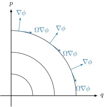
Gradient of the constraint function $\phi$ orthogonal and $\Omega$-orthogonal to constant surfaces of $\phi(q, p) = p - \sqrt{p_{0}^{2} - q^{2}}$ for $p_{0} \in \{ 1, 2, 3 \}$.
Let us emphasize that in contrast to standard projection methods, where the solution is projected orthogonal to the constrained submanifold, along the gradient of $\phi$, here the projection has to be $\Omega$-orthogonal, where $\Omega$ is the canonical symplectic matrix
\[\begin{equation}\label{eq:canonical-symplectic-matrix} \Omega = \begin{pmatrix} \mathbb{0} & - \mathbb{1} \\ \mathbb{1} & \hphantom{-} \mathbb{0} \end{pmatrix} . \end{equation}\]
That is, denoting by $\lambda$ the Lagrange multiplier, the projection step is given by $\Omega^{-1} \nabla \phi^{T} \lambda$ instead of an orthogonal projection $\nabla \phi^{T} \lambda$.
Let us also note that, practically speaking, the momenta $p_{n}$ and $p_{n+1}$ are merely treated as intermediate variables much like the internal stages of a Runge-Kutta method. The Lagrange multiplier $\lambda$, on the other hand, is determined in different ways for the different methods and can be the same or different in the perturbation and the projection. It thus takes the role of an internal variable only for the standard, symmetric projection and midpoint projection, but not for the symplectic projection.
Geometric Aside: Projected Fibre Derivatives
In the following, we will try to underpin the construction of the various projection methods with some geometric ideas. We already mentioned several times that the position-momentum form of the variational integrator \eqref{eq:vi-position-momentum-form} suffers from the problem that it does not preserve the constraint submanifold $\Delta$ defined in \eqref{eq:constraint-submanifold}. That is, even though it is applied to a point in $i(\Delta)$, it usually returns a point in $\cb{\mf{M}}$, but outside of $i(\Delta)$. In order to understand the reason for this, let us define $\Delta_{\mf{M}}^{-}$ and $\Delta_{\mf{M}}^{+}$ as the subsets of $\mf{M} \times \mf{M}$ which are mapped into the constraint submanifold $i(\Delta)$ by the discrete fibre derivatives $\mathbb{F}^{-} L_{d}$ and $\mathbb{F}^{+} L_{d}$, respectively, i.e.,
\[\begin{equation}\label{eq:constraint-submanifold_QxQ} \begin{aligned} \Delta_{\mf{M}}^{-} &= \{ (q_{n}, q_{n+1}) \in \mf{M} \times \mf{M} \, \big\vert \, \mathbb{F}^{-} L_{d} (q_{n}, q_{n+1}) = (q_{n}, p_{n}) \in i(\Delta) \big\} , \\ \Delta_{\mf{M}}^{+} &= \{ (q_{n}, q_{n+1}) \in \mf{M} \times \mf{M} \, \big\vert \, \mathbb{F}^{+} L_{d} (q_{n}, q_{n+1}) = (q_{n+1}, p_{n+1}) \in i(\Delta) \big\} , \end{aligned} \end{equation}\]
or more explicitly,
\[\begin{equation}\label{eq:constraint-submanifold_QxQ_coordinates} \begin{aligned} \Delta_{\mf{M}}^{-} &= \{ (q_{n}, q_{n+1}) \in \mf{M} \times \mf{M} \, \big\vert \, - D_{1} L_{d} (q_{n}, q_{n+1}) = \vartheta(q_{n}) \big\} , \\ \Delta_{\mf{M}}^{+} &= \{ (q_{n}, q_{n+1}) \in \mf{M} \times \mf{M} \, \big\vert \, D_{2} L_{d} (q_{n}, q_{n+1}) = \vartheta(q_{n+1}) \big\} . \end{aligned} \end{equation}\]
A sufficient condition for the position-momentum form of the variational integrator \eqref{eq:vi-position-momentum-form} to preserve the constraint submanifold \eqref{eq:constraint-submanifold} would be that $\Delta_{\mf{M}}^{-}$ and $\Delta_{\mf{M}}^{+}$ are identical. In principle, slightly weaker necessary conditions can be formulated, however in practice it is unclear how to prove any of these conditions and in general they are not satisfied.
In order to construct a modified algorithm which does preserve the constraint submanifold, we compose the discrete fibre derivatives $\mathbb{F}^{\pm}$ with appropriate projections $\mathbb{P}^{\pm}$,
\[\begin{equation}\label{eq:position_momentum_projection} \begin{aligned} (q_{n}, p_{n }) &= \big( \mathbb{P}^{-} \circ \mathbb{F}^{-} L_{d} \big) (q_{n}, q_{n+1}) = \mathbb{P}_{\lambda_{n}^{-}}^{-} \big( q_{n}, - D_{1} L_{d} (q_{n}, q_{n+1}) \big) , \\ (q_{n+1}, p_{n+1}) &= \big( \mathbb{P}^{+} \circ \mathbb{F}^{+} L_{d} \big) (q_{n}, q_{n+1}) = \mathbb{P}_{\lambda_{n+1}^{+}}^{+} \big( q_{n+1}, D_{2} L_{d} (q_{n}, q_{n+1}) \big) , \end{aligned} \end{equation}\]
so that they take any point in $\mf{M} \times \mf{M}$ to the constraint submanifold $\Delta$. The Lagrange multiplier $\lambda$ is indicated as subscript and implicitly determined by requiring that the constraint $\phi$ is satisfied by the projected values of $q$ and $p$. These projected fibre derivatives will not be a fibre-preserving map anymore, but they will change both $q$ and $p$. Noting that the nullspace of $\mathbb{P}_{\lambda}$ is the span of $\Omega^{-1} \nabla \phi$, a natural candidate for the projection $\mathbb{P}_{\lambda}$ is given by
\[\begin{equation}\label{eq:projector} \begin{aligned} \mathbb{P}_{\lambda}^{\pm} (q, p) : (q, p) &= (q, p) \pm h \, \Omega^{-1} \nabla \phi^{T} (q, p) \lambda , & 0 &= \phi(q, p) , \end{aligned} \end{equation}\]
so that $( \mathbb{P}^{-} \circ \mathbb{F}^{-} L_{d} ) (q_{n}, q_{n+1})$ explicitly reads
\[\begin{aligned} q_{n} &= q_{n} - h \, \phi_{p}^{T} (q_{n}, p_{n}) \lambda_{n}^{-} , \\ p_{n} &= - D_{1} L_{d} (q_{n}, q_{n+1}) + h \, \phi_{q}^{T} (q_{n}, p_{n}) \lambda_{n}^{-} , \\ 0 &= \phi(q_{n}, p_{n}) , \end{aligned}\]
and $( \mathbb{P}^{+} \circ \mathbb{F}^{+} L_{d} ) (q_{n}, q_{n+1})$ explicitly reads
\[\begin{aligned} q_{n+1} &= q_{n+1} + h \, \phi_{p}^{T} (q_{n+1}, p_{n+1}) \lambda_{n+1}^{+} , \\ p_{n+1} &= D_{2} L_{d} (q_{n}, q_{n+1}) - h \, \phi_{q}^{T} (q_{n+1}, p_{n+1}) \lambda_{n+1}^{+} , \\ 0 &= \phi(q_{n+1}, p_{n+1}) . \end{aligned}\]
The signs in front of the projections have been chosen in correspondence with the signs of the discrete forces in [9], Chapter 3. With these projections we obtain all of the algorithms introduced in the following sections, except for the midpoint projection, in a similar fashion to the definition of the position-momentum form of the variational integrator \eqref{eq:vi-position-momentum-form}, as a map $\Delta \rightarrow \Delta$ which can formally be written as
\[\begin{equation}\label{eq:projection-composition-map} \Phi_{h} = \big( \pi_{\Delta} \circ \mathbb{P}^{+} \circ \mathbb{F}^{+} L_{d} \big) \circ \big( \pi_{\Delta} \circ \mathbb{P}^{-} \circ \mathbb{F}^{-} L_{d} \big)^{-1} . \end{equation}\]
In total, we obtain algorithms which map $q_{n}$ into $q_{n+1}$ via the steps
\[\Delta \xrightarrow{\pi_{\Delta}^{-1}} i(\Delta) \xrightarrow{(\mathbb{P}^{-})^{-1}} \cb{\mf{M}} \xrightarrow{(\mathbb{F}^{-} L_{d})^{-1}} \mf{M} \times \mf{M} \xrightarrow{\mathbb{F}^{+} L_{d}} \cb{\mf{M}} \xrightarrow{\mathbb{P}^{+}} i(\Delta) \xrightarrow{\pi_{\Delta}} \Delta ,\]
where $\pi_{\Delta}^{-1}$ is identical to the inclusion \eqref{eq:dirac-inclusion}. The difference of the various algorithms lies in the choice of $\lambda_{n}^{-}$ and $\lambda_{n+1}^{+}$ as follows
| Projection | $\lambda_{n}^{-}$ | $\lambda_{n+1}^{+}$ |
|---|---|---|
| Standard | $0$ | $\lambda_{n+1}$ |
| Symplectic | $\lambda_{n}$ | $R (\infty) \, \lambda_{n+1\hphantom{/2}}$ |
| Symmetric | $\lambda_{n+1/2}$ | $R (\infty) \, \lambda_{n+1/2}$ |
| Midpoint | $\lambda_{n+1/2}$ | $R (\infty) \, \lambda_{n+1/2}$ |
For the symmetric, symplectic and midpoint projections, it is important to adapt the sign in the projection according to the stability function $R(\infty)$ of the basic integrator (for details see e.g. [29]). For the methods we are interested in, namely Runge-Kutta methods, the stability function is given by $R(z) = 1 + z b^{T} (\identity - zA)^{-1} e$ with $e = (1, 1, ..., 1)^{T} \in \mathbb{R}^{s}$, and we have $\abs{R(\infty)}=1$ or, more specifically, for Gauss-Legendre methods $R(\infty) = (-1)^{s}$ and for partitioned Gauss-Lobatto IIIA-IIIB and IIIB-IIIA methods we have $R(\infty) = (-1)^{s-1}$.
Let us remark that for the standard projection, the basic integrator and the projection step can be applied independently. Similarly, for the symplectic projection, the three steps, namely perturbation, numerical integrator, and projection, decouple and can be solved consecutively, as we use different Lagrange multipliers $\lambda_{n}$ in the perturbation and $\lambda_{n+1}$ in the projection. For the symmetric projection and the midpoint projection, however, this is not the case. There, we used the same Lagrange multiplier $\lambda_{n+1/2}$ in both the perturbation and the projection, so that the whole system has to be solved at once, which is more costly. This also implies that for the projection methods where $\lambda_{n}^{-}$ and $\lambda_{n+1}^{+}$ are the same (possibly up to a sign due to $R(\infty)$), strictly speaking we cannot write the projected algorithm in terms of a composition of two steps as we did in \eqref{eq:projection-composition-map}. Instead the whole algorithm has to be treated as one nonlinear map. The idea of the construction of the methods is still the same, though. Only the midpoint projection needs special treatment. There, the operator $\mathbb{P}_{\lambda}$ is defined in a slightly more complicated way than in \eqref{eq:projector}, using different arguments in the projection step, which does not quite fit the general framework outlined here.
Standard Projection
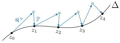
Illustration of the standard projection method: The solution is projected to the constraint submanifold $\Delta$ after each step of the numerical integrator $\Psi_{h}$.
The standard projection method [[5], Section IV.4] is the simplest projection method. Starting from $q_{n}$, we use the continuous fibre derivative \eqref{eq:fibre-derivative-general} to compute $p_{n} = \vartheta (q_{n})$. Then we apply some symplectic one-step method $\Psi_{h}$ to $z_{n} = (q_{n}, p_{n})$ to obtain an intermediate solution $z_{n+1}$,
\[\bar{z}_{n+1} = \Psi_{h} (z_{n}) ,\]
which is projected onto the constraint submanifold \eqref{eq:constraint-submanifold} by
\[\begin{equation}\label{eq:orthogonal_projection} z_{n+1} = \bar{z}_{n+1} + h \, \Omega^{-1} \nabla \phi^{T} (z_{n+1}) \lambda_{n+1} , \end{equation}\]
enforcing the constraint
\[0 = \phi (z_{n+1}) .\]
This projection method, combined with the variational integrator in position-momentum form \eqref{eq:vi-position-momentum-form}, is not symmetric, and therefore not reversible. Moreover, it exhibits a drift of the energy, as has been observed before, e.g., for holonomic constraints [[28], [27], [5]].
Symmetric Projection
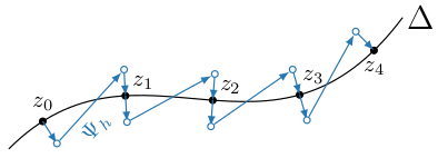
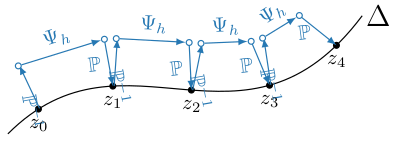
Illustration of the symmetric projection method: The solution is first perturbed off the constraint submanifold $\Delta$, then one step of the numerical integrator $\Psi_{h}$ is performed, and the result is projected back onto $\Delta$.
To overcome the shortcomings of the standard projection, we consider a symmetric projection of the variational Runge-Kutta integrators following [28], [27] and [29], see also [5], Section V.4.1. Here, one starts again by computing the momentum $p_{n}$ as a function of the coordinates $q_{n}$ according to the continuous fibre derivative, which can be expressed with the constraint function as
\[\begin{equation}\label{eq:symmetric-symplectic-projection} 0 = \phi (z_{n}) . \end{equation}\]
Then the initial value $z_{n}$ is first perturbed,
\[\begin{equation}\label{eq:symmetric-projection-pre} \bar{z}_{n} = z_{n} + h \, \Omega^{-1} \nabla \phi^{T} (z_{n}) \, \lambda_{n+1/2} , \end{equation}\]
followed by the application of some one-step method $\Psi_{h}$,
\[\bar{z}_{n+1} = \Psi_{h} (\bar{z}_{n}) ,\]
and a projection of the result onto the constraint submanifold,
\[\begin{equation}\label{eq:symmetric_projection_post} z_{n+1} = \bar{z}_{n+1} + h \, R(\infty) \, \Omega^{-1} \nabla \phi^{T} (z_{n+1}) \lambda_{n+1/2} , \end{equation}\]
which enforces the constraint
\[0 = \phi (z_{n+1}) .\]
Here, it is important to note that Lagrange multiplier $\lambda_{n+1/2}$ is the same in both the perturbation and the projection step, and to account for the stability function $R(\infty)$ of the basic integrator, as mentioned before. The algorithm composed of the symmetric projection and some symmetric variational integrator in position-momentum form, constitutes a symmetric map
\[\Phi_{h} : q_{n} \mapsto q_{n+1} ,\]
where, from a practical point of view, $p_{n}$, $p_{n+1}$ and $\lambda_{n+1/2}$ are treated as intermediate variables. Unfortunately, the method is not symplectic but instead satisfies the relation
\[\begin{multline}\label{eq:symmetric-projection-symplecticity-condition} \dfrac{1}{2} \bar{\Omega}_{ij} (q_{n}) \, \big( \ext q_{n}^{i} \wedge \ext q_{n}^{j} - h^{2} \, \ext \lambda_{n+1/2}^{i} \wedge \ext \lambda_{n+1/2}^{j} \big) - h^{2} \lambda_{n+1/2}^{k} \vartheta_{k,ij} (q_{n}) \, \ext q_{n}^{i} \wedge \ext \lambda_{n+1/2}^{j} = \\ = \dfrac{1}{2} \bar{\Omega}_{ij} (q_{n+1}) \, \big( \ext q_{n+1}^{i} \wedge \ext q_{n+1}^{j} - h^{2} \, \ext \lambda_{n+1/2}^{i} \wedge \ext \lambda_{n+1/2}^{j} \big) - h^{2} \lambda_{n+1/2}^{k} \vartheta_{k,ij} (q_{n+1}) \, \ext q_{n+1}^{i} \wedge \ext \lambda_{n+1/2}^{j} . \end{multline}\]
For certain systems, this method can even be shown to be symplectic. In general, though, it is not symplectic. Nevertheless, it tends to perform very well in long-time simulations.
Symplectic Projection
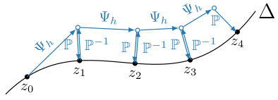
Illustration of the post projection method. Starting on the constraint submanifold $\Delta$, the numerical integrator $\Psi_{h}$ moves the solution away from $\Delta$ in the first step. After each step, the solution is projected back onto $\Delta$, but the perturbation at the beginning of each consecutive step is exactly the inverse of the previous projection, so that, practically speaking, the solution is projected back onto $\Delta$ only for output purposes.
In the symplectic projection, we modify the perturbation \eqref{eq:symmetric-projection-pre} to use the Lagrange multiplier at the previous time step, $\lambda_{n}$, instead of $\lambda_{n+1}$. As before, we assum the initial condition $z_{n}$ satisfies the constraint,
\[\begin{equation}\label{eq:symplectic-projection-pre-constraint} 0 = \phi (z_{n}) . \end{equation}\]
The initial condition is perturbed, using the Lagrange multiplier $\lambda_{n}$,
\[\begin{equation}\label{eq:symplectic-projection-pre} \bar{z}_{n} = z_{n} + h \, \Omega^{-1} \nabla \phi^{T} (z_{n}) \, \lambda_{n} . \end{equation}\]
Then the usual one-step method $\Psi_{h}$ is applied,
\[\bar{z}_{n+1} = \Psi_{h} (\bar{z}_{n}) ,\]
and the result is projected onto the constraint submanifold using the Lagrange multiplier $\lambda_{n+1}$,
\[\begin{equation}\label{eq:symplectic-projection-post} z_{n+1} = \bar{z}_{n+1} + h \, R(\infty) \, \Omega^{-1} \nabla \phi^{T} (z_{n+1}) \lambda_{n+1} , \end{equation}\]
in order to enforce the constraint
\[\begin{equation}\label{eq:symplectic-projection-post-constraint} 0 = \phi (z_{n+1}) . \end{equation}\]
The symplecticity condition \eqref{eq:symmetric-projection-symplecticity-condition} is modified as follows,
\[\begin{multline}\label{eq:symplectic_projection_symplecticity_condition} \dfrac{1}{2} \bar{\Omega}_{ij} (q_{n}) \, \big( \ext q_{n}^{i} \wedge \ext q_{n}^{j} - h^{2} \, \ext \lambda_{n}^{i} \wedge \ext \lambda_{n}^{j} \big) - h^{2} \lambda_{n}^{k} \vartheta_{k,ij} (q_{n}) \, \ext q_{n}^{i} \wedge \ext \lambda_{n}^{j} = \\ = \dfrac{1}{2} \bar{\Omega}_{ij} (q_{n+1}) \, \big( \ext q_{n+1}^{i} \wedge \ext q_{n+1}^{j} - h^{2} \, \ext \lambda_{n+1}^{i} \wedge \ext \lambda_{n+1}^{j} \big) \\ - h^{2} \lambda_{n+1/2}^{k} \vartheta_{k,ij} (q_{n+1}) \, \ext q_{n+1}^{i} \wedge \ext \lambda_{n+1}^{j} , \end{multline}\]
implying the conservation of a modified symplectic form $\omega_{\lambda}$ defined on an extended phasespace $\mf{M} \times \mathbb{R}^{d}$ with coordinates $(q, \lambda)$ by
\[\begin{equation}\label{eq:symplectic_projection_two_form} \omega_{\lambda} = \dfrac{1}{2} \bar{\Omega}_{ij} (q) \, \ext q^{i} \wedge \ext q^{j} - \dfrac{h^{2}}{2} \bar{\Omega}_{ij} (q) \, \ext \lambda^{i} \wedge \ext \lambda^{j} - h^{2} \lambda^{k} \vartheta_{k,ij} (q) \, \ext q^{i} \wedge \ext \lambda^{j} , \end{equation}\]
with matrix representation
\[\Omega_{\lambda} = \begin{pmatrix} \bar{\Omega} & - h^{2} \lambda \cdot \vartheta_{qq} \\ h^{2} \lambda \cdot \vartheta_{qq} & - h^{2} \bar{\Omega} \\ \end{pmatrix} .\]
This corresponds to a modified one-form $\vartheta_{\lambda}$, such that $\omega_{\lambda} = \ext \vartheta_{\lambda}$, given by
\[\begin{equation}\label{eq:symplectic_projection_one_form} \vartheta_{\lambda} = ( \vartheta_{i} (q) - h \, \lambda^{k} \vartheta_{k,i} (q) ) \, ( \ext q^{i} - h \, \ext \lambda^{i} ) \end{equation}\]
As noted by [29], the modified perturbation \eqref{eq:symplectic-projection-pre-constraint}-\eqref{eq:symplectic-projection-pre} can be viewed as a change of variables from $(q, \lambda)$ on $\mf{M} \times \mathbb{R}^{d}$ to $(q, p)$ on $\cb{\mf{M}}$, and the projection \eqref{eq:symplectic-projection-post}-\eqref{eq:symplectic-projection-post-constraint} as a change of variables back from $(q, p)$ to $(q, \lambda)$. The symplectic form $\omega_{\lambda}$ on $\mf{M} \times \mathbb{R}^{d}$ thus corresponds to the pullback of the canonical symplectic form $\omega$ on $\cb{\mf{M}}$ by this variable transformation.
Let us note that the sign in in front of the projection in \eqref{eq:symplectic-projection-post}, given by the stability function of the basic integrator, has very important implications on the nature of the algorithm. If it is the same as in \eqref{eq:symplectic-projection-pre}, the character of the method is very similar to the symmetric projection method described before. If the sign is the opposite of the one in \eqref{eq:symplectic-projection-pre}, like for Gauss-Legendre Runge-Kutta methods with an odd number of stages, the perturbation reverses the projection of the previous step, so that we effectively apply the post-projection method of [32]. That is, the projected integrator $\Phi_{h}$ is conjugate to the unprojected integrator $\Psi_{h}$ by
\[\Phi_{h} = \mathbb{P}^{-1} \circ \Psi_{h} \circ \mathbb{P} ,\]
so that the following diagram commutes

and the projection is effectively only applied for the output of the solution, but the actual advancement of the solution in time happens outside of the constraint submanifold. In other words, applying $n$ times the algorithm $\Phi_{h}$ to a point $(q_{0}, 0)$ is equivalent to applying the perturbation $\mathbb{P}^{-1}$, then applying $n$ times the algorithm $\Psi_{h}$ and projecting the result with $\mathbb{P}$.
Potentially, this might degrade the performance of the algorithm. If the accumulated global error drives the solution too far away from the constraint submanifold, the projection step might not have a solution anymore. Interestingly, however, post-projected Gauss-Legendre Runge-Kutta methods retain their optimal order of $2s$ [[32]]. Moreover, for methods with an odd number of stages, the global error of the unprojected solution is $\mathcal{O}(h^{s+1})$, compared to $\mathcal{O}(h^{s})$ for methods with an even number of stages. In practice this seems to be at least part of the reason of the good long-time stability of these methods.
Midpoint Projection
For certain variational Runge-Kutta methods, we can also modify the symmetric projection in a different way in order to obtain a symplectic projection, namely by evaluating the projection at the midpoint
\[\begin{aligned} \bar{z}_{n+1/2} &= (\bar{q}_{n+1/2}, \bar{p}_{n+1/2}) , & \bar{q}_{n+1/2} &= \tfrac{1}{2} \big( \bar{q}_{n} + \bar{q}_{n+1} \big) , & \bar{p}_{n+1/2} &= \tfrac{1}{2} \big( \bar{p}_{n} + \bar{p}_{n+1} \big) , \end{aligned}\]
so that the projection algorithm is modified as follows. As always, the initial condition is expected to satisfy the constraint,
\[\begin{equation}\label{eq:midpoint_projection_pre_constraint} 0 = \phi (z_{n}) . \end{equation}\]
For the perturbation of the initial condition,
\[\begin{equation}\label{eq:midpoint_projection_pre} \bar{z}_{n} = z_{n} + h \, \Omega^{-1} \nabla \phi^{T} (\bar{z}_{n+1/2}) \, \lambda_{n+1/2} , \end{equation}\]
the gradient of the constraint is evaluated at the midpoint $\bar{z}_{n+1/2}$. A one step method is applied,
\[\bar{z}_{n+1} = \Psi_{h} (z_{\bar{z}}) ,\]
and the result is projected, again evaluating the gradient of $\phi$ at the midpoint $\bar{z}_{n+1/2}$,
\[\begin{equation}\label{eq:midpoint_projection_post} z_{n+1} = \bar{z}_{n+1} + h \, R(\infty) \, \Omega^{-1} \nabla \phi^{T} (z_{n+1/2}) \lambda_{n+1/2} , \end{equation}\]
in order to force the solution to satisfy the constraint,
\[\begin{equation}\label{eq:symplectic_projection_midpoint_post_constraint} 0 = \phi (z_{n+1}) . \end{equation}\]
For certain systems, this method can be shown to be symplectic with respect to the original noncanonical symplectic form on $\mf{M}$ if the integrator $\Psi_{h}$ is a symmetric, symplectic Runge-Kutta method with an odd number of stages $s$, for which the central stage with index $(s+1)/2$ corresponds to $z_{n+1/2}$. This is obviously the case for the implicit midpoint rule, that is the Gauss-Legendre Runge-Kutta method with $s=1$, but unfortunately not for higher-order Gauss-Legendre or for Gauss-Lobatto methods. However, following [35] and [36], higher-order methods similar to Gauss-Legendre methods but satisfying the requested property can be obtained. See for example the method with three stages, implemented as SRK3.
Internal Stage Projection
TODO