Variational Integrators

The basic idea of variational integrators is to construct a discrete counterpart to a particular mechanical system instead of directly discretising its equations of motion. This means that the fundamental building blocks of classical mechanics, namely the action functional, the Lagrangian, the variational principle, and the Noether theorem, all have discrete equivalents. The application of the discrete variational principle to the discrete action then leads to discrete Euler-Lagrange equations. The evolution map that corresponds to the discrete Euler-Lagrange equations is what is called a variational integrator. The discrete Noether theorem can be used to relate symmetries of the discretised system to discrete momenta that are in principle exactly preserved by this integrator.

With standard numerical methods, one approximately solves the exact equations of some system. In a sense, the idea of variational integrators is to exactly solve the equations of an approximate system.

The seminal work in the development of a discrete equivalent of classical mechanics was presented by [[10], [10]]. His method, based on a discrete variational principle, leads to symplectic integration schemes that automatically preserve constants of motion [[11], [12]]. A comprehensive review of discrete mechanics can be found in [[9]], including a thorough account on the historical development. The discrete version of Hamilton's phasespace action principle is presented in [[13]].

Discretisation of the Action

The derivation of the discrete theory follows along the lines of the derivation of the continuous theory. The starting point is the discretisation of the space of paths $\mathcal{Q} ( \mf{M} )$ that connect two points in $\mf{M}$,

\[\mathcal{Q} ( \mf{M} ) = \big\{ q : \mathcal{I} \rightarrow \mf{M} \; \big\vert \; \mathcal{I} \subset \mathbb{R} \; \text{smooth and bounded} \big\} .\]

Therefore we divide each time interval $\mathcal{I}$ into an equidistant, monotonic sequence $\{ t_{n} \}_{n=0}^{N}$ and defined the discrete path space as

\[\mathcal{Q}_{d} ( \mf{M} ) = \big\{ q_{d} : \{ t_{n} \}_{n=0}^{N} \rightarrow \mf{M} \big\} .\]

The space $\mathcal{Q}_{d} ( \mf{M} )$ contains all possible discrete trajectories $q_{d}$ in $\mf{M}$ and is isomorphic to $\mf{M} \times ... \times \mf{M}$ ($N+1$ copies),

\[\mathcal{Q}_{d} ( \mf{M} ) \cong \bigtimes_{N+1} \mf{M} .\]

Therefore $\mathcal{Q}_{d} ( \mf{M} )$ constitutes a finite-dimensional approximation of the infinite-dimensional space $\mathcal{Q} ( \mf{M} )$. Note that $\mathcal{Q}_{d}$ is not a subspace of $\mathcal{Q}$. Fixing an interval $[0, T]$, so that

\[\{ t_{n} \}_{n=0}^{N} = \{ t_{n} = nh \; \vert \; n = 0, ..., N , \; Nh = T \} \subset \mathbb{R} ,\]

is an increasing sequence of time points and $h$ is the discrete time step, the discrete equivalent of the space of curves from $q_{0}$ to $q_{N}$,

\[\mathcal{Q} ( q_{0}, q_{N}, [0, T] ) = \big\{ q : [0, T] \rightarrow \mf{M} \; \big\vert \; q(0) = q_{0}, \, q(T) = q_{N} \big\} \subset \mathcal{Q} ( \mf{M} ) ,\]

is the space that contains all discrete trajectories with fixed endpoints $q_{0}$ and $q_{N}$, defined as

\[\mathcal{Q}_{d} ( q_{0}, q_{N}, \{ t_{n} \}_{n=0}^{N} ) = \big\{ q_{d} : \{ t_{n} \}_{n=0}^{N} \rightarrow \mf{M} \; \big\vert \; q(t_{0}) = q_{0}, q(t_{N}) = q_{N} \big\} \subset \mathcal{Q}_{d} ( \mf{M} ) .\]

The discrete trajectory can be written as $q_{d} = \{ q_{n} \}_{n=0}^{N}$, where $q_{n}$ denotes the generalised coordinates at time $t_{n}$. The space $\mathcal{Q}_{d} ( q_{0}, q_{N}, \{ t_{n} \}_{n=0}^{N} )$ is a finite-dimensional approximation of $\mathcal{Q} ( q_{0}, q_{N}, [0, T] )$. In the following, we will use piecewise linear Lagrange polynomials to approximate the trajectory $q(t)$, that is

\[\begin{equation}\label{eq:vi-linear-interpolation} q_{h} (t) \big\vert_{[t_{n}, t_{n+1}]} = q_{n} \dfrac{t_{n+1} - t}{t_{n+1} - t_{n}} + q_{n+1} \dfrac{t - t_{n}}{t_{n+1} - t_{n}} . \end{equation}\]

The next step is to choose a quadrature rule which determines the discrete action. While the continuous action is a map

\[\mathcal{A} : \mathcal{Q} ( q_{0}, q_{N}, [0, T] ) \rightarrow \mathbb{R} ,\]

assigning real values to each path $q(t)$, the discrete action is a map

\[\mathcal{A}_{d} : \mathcal{Q}_{d} ( q_{0}, q_{N}, \{ t_{n} \}_{n=0}^{N} ) \rightarrow \mathbb{R} ,\]

assigning real values to each discrete path $q_{d}$. Once we obtained the discrete action, everything else follows in a straight forward and systematic way from Hamilton's principle of stationary action, so that these choices are determining the form of the discrete equations of motion.

After we fix the sequence $\{ t_{n} \}_{n=0}^{N}$, the continuous action can be written as

\[\mathcal{A} [q] = {\sum}_{n=0}^{N-1} \int_{t_{n}}^{t_{n+1}} L (q, \dot{q}) \, dt .\]

The terms of the sum are called the \emph{exact discrete Lagrangian},

\[L_{d}^{\mathrm{e}} (q_{n}, q_{n+1}) = \int_{t_{n}}^{t_{n+1}} L \big( q_{n,n+1} (t), \, \dot{q}_{n,n+1} (t) \big) \, dt ,\]

which is defined as a function of two consecutive points on the discrete trajectory $q_{d} = \{ q_{n} \}_{n=0}^{N}$. Here, $q_{n,n+1} (t)$ denotes the solution of the continuous Euler-Lagrange equations in the interval $[t_{n}, t_{n+1}]$ satisfying the boundary conditions $q_{n,n+1} (t_{n}) = q_{n}$ and $q_{n,n+1} (t_{n+1}) = q_{n+1}$, with $q_{n}$ denoting the generalised coordinates at time $t_{n}$ and $\dot{q}_{n}$ the generalised velocities at time point $t_{n}$. In practice, the exact discrete Lagrangian cannot be computed exactly, which means we have to approximate it,

\[L_{d} (q_{n}, q_{n+1}) \approx \int_{t_{n}}^{t_{n+1}} L \big( q_{n,n+1} (t), \, \dot{q}_{n,n+1} (t) \big) \, dt .\]

That is, we have to approximate the trajectory $q(t)$, the velocity $\dot{q}(t)$ and the integral. This approximation leads to the discrete Lagrangian, given as

\[\begin{equation}\label{eq:vi-quadrature} L_{d} (q_{n}, q_{n+1}) = h \sum \limits_{i=1}^{s} b_{i} \, L \big( q_{h} (t_{n} + c_{i} h), \, \dot{q}_{h} (t_{n} + c_{i} h) \big) , \end{equation}\]

where $q_{n} = q_{h} (t_{n})$ and $q_{n+1} = q_{h} (t_{n+1})$. The discrete action thus becomes merely a sum over the time index of discrete Lagrangians

\[\begin{equation}\label{eq:vi-action} \mathcal{A}_{d} [q_{d}] = \sum \limits_{n=0}^{N-1} L_{d} (q_{n}, q_{n+1}) , \end{equation}\]

which defines a map $\mathcal{A}_{d} : \mathcal{Q}_{d} ( q_{0}, q_{N}, \{ t_{n} \}_{n=0}^{N} ) \rightarrow \mathbb{R}$. In order to obtain the discrete Lagrangian, the generalised velocities are often discretised by simple finite-difference expressions\footnote{ In the first term of the trapezoidal rule \eqref{eq:vi-trapezoidal}, this corresponds to a forward finite-difference, in the second term to a backward finite-difference, and in the midpoint rule \eqref{eq:vi-midpoint} to a centred finite-difference. }, i.e.,

\[\dot{q} (t) \approx \dfrac{q_{n+1} - q_{n}}{h} \hspace{3em} \text{for} \hspace{3em} t \in [ t_{n} , t_{n+1} ] . \]

This corresponds to approximating the trajectory $q(t)$ between $t_{n}$ and $t_{n+1}$ by linear interpolation between $q_{n}$ and $q_{n+1}$ like in \eqref{eq:vi-linear-interpolation} and taking the derivative of $q_{h} (t)$ with respect to $t$. The quadrature is most often realised by either the trapezoidal rule ($c_{1} = 0$, $c_{2} = 1$),

\[\begin{equation}\label{eq:vi-trapezoidal} L_{d}^{\text{tr}} (q_{n}, q_{n+1}) = \dfrac{h}{2} \, L \bigg( q_{n}, \dfrac{q_{n+1} - q_{n}}{h} \bigg) + \dfrac{h}{2} \, L \bigg( q_{n+1}, \dfrac{q_{n+1} - q_{n}}{h} \bigg) , \end{equation}\]

or the midpoint rule ($c_{1} = 1/2$),

\[\begin{equation}\label{eq:vi-midpoint} L_{d}^{\text{mp}} (q_{n}, q_{n+1}) = h \, L \bigg( \dfrac{q_{n} + q_{n+1}}{2}, \dfrac{q_{n+1} - q_{n}}{h} \bigg) . \end{equation}\]

The configuration manifold of the discrete theory is still $\mf{M}$, but the discrete state space is $\mf{M} \times \mf{M}$ instead of $\tb{\mf{M}}$, such that the discrete Lagrangian $L_{d}$ is a function

\[\begin{equation}\label{eq:vi-discrete_lagrangian} L_{d} : \mf{M} \times \mf{M} \rightarrow \mathbb{R} , \end{equation}\]

mapping two points on the discrete trajectory into the real numbers.

Discrete Euler-Lagrange Equations

The discrete trajectories $q_{d} = \{ q_{n} \}_{n=0}^{N}$ are required to satisfy a discrete version of Hamilton's principle of stationary action

\[\delta \mathcal{A}_{d} [q_{d}] = \delta \sum \limits_{n=0}^{N-1} L_{d} (q_{n}, q_{n+1}) = 0 .\]

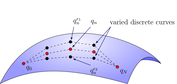
As each point $q_{n}$ of the discrete trajectory takes continuous values, we consider variations as as one-parameter families of transformations, that is families of paths $q_{d}^{\epsilon} = \{ q_{n}^{\epsilon} \}_{n=0}^{N} \in \mathcal{Q}_{d} ( q_{0}, q_{N}, \{ t_{n} \}_{n=0}^{N} )$ which contain the solution path $q_{d}$ for $\epsilon=0$. The variations of $q_{d}$ are contained in the tangent space $\tb[q_{d}]{\mathcal{Q}_{d} ( q_{0}, q_{N}, \{ t_{n} \}_{n=0}^{N} )}$ to $\mathcal{Q}_{d} ( q_{0}, q_{N}, \{ t_{n} \}_{n=0}^{N} )$ at $q_{d}$. It is defined as the set of maps

\[\begin{aligned} v_{q_{d}} : \{ t_{n} \}_{n=0}^{N} &\rightarrow \tb{\mf{M}} & & \text{such that} & \pi_{\mf{M}} \circ v_{q_{d}} &= q_{d} & & \text{and} & v (t_{0}) = v (t_{N}) &= 0 , \end{aligned}\]

where $\pi_{\mf{M}}$ is the canonical projection $\pi_{\mf{M}} : \tb{\mf{M}} \rightarrow \mf{M}$ and local coordinates are given by

\[v_{q_{d}} = \{ (q_{n}, v_{n}) \}_{n=0}^{N} .\]

In particular, a discrete variation $v_{q_{d}}$ of the discrete path $q_{d}$ is defined as

\[v_{q_{d}} = \dfrac{d}{d\epsilon} q_{d}^{\epsilon} \bigg\vert_{\epsilon=0} .\]

By identifying $\delta \equiv d / d\epsilon \big\vert_{\epsilon=0}$, we can also denote the variation by $v_{q_{d}} = \delta q_{d}$. In analogy to the continuous setting, the variation of the discrete action can be written as

\[\delta \mathcal{A}_{d} [q_{d}] = \dfrac{d}{d\epsilon} \mathcal{A}_{d} [q_{d}^{\epsilon}] \bigg\vert_{\epsilon=0} = \ext \mathcal{A}_{d} [q_{d}] \cdot v_{q_{d}} ,\]

which explicitly computed becomes

\[\begin{equation}\label{eq:vi-variation_01} \ext \mathcal{A}_{d} [q_{d}] \cdot v_{q_{d}} = \sum \limits_{n=0}^{N-1} \big[ D_{1} \, L_{d} (q_{n}, q_{n+1}) \cdot v_{n} + D_{2} \, L_{d} (q_{n}, q_{n+1}) \cdot v_{n+1} \big] , \end{equation}\]

where $D_{i}$ denotes the derivative with respect to to the $i$th argument (slot derivative). What follows corresponds to a discrete integration by parts, i.e., a reordering of the summation. The $n=0$ term is separated from the first part of the sum and the $n=N-1$ term is separated from the second part

\[\begin{equation}\label{eq:vi-variation_02} \begin{aligned} \ext \mathcal{A}_{d} [q_{d}] \cdot v_{q_{d}} \nonumber = D_{1} \, L_{d} (q_{0}, q_{1}) \cdot v_{0} &+ \sum \limits_{n=1}^{N-1} D_{1} \, L_{d} (q_{n}, q_{n+1}) \cdot v_{n} \\ &+ \sum \limits_{n=0}^{N-2} D_{2} \, L_{d} (q_{n}, q_{n+1}) \cdot v_{n+1} + D_{2} \, L_{d} (q_{N-1}, q_{N}) \cdot v_{N} . \end{aligned} \end{equation}\]

As the variations at the endpoints are kept fixed, $v_{0} = v (t_{0}) = 0$ as well as $v_{N} = v (t_{N}) = 0$, the corresponding terms vanish. At last, the summation range of the second sum is shifted upwards by one with the arguments of the discrete Lagrangian adapted correspondingly

\[\begin{equation}\label{eq:vi-variation_03} \ext \mathcal{A}_{d} [q_{d}] \cdot v_{q_{d}} = \sum \limits_{n=1}^{N-1} \big[ D_{1} \, L_{d} (q_{n}, q_{n+1}) + D_{2} \, L_{d} (q_{n-1}, q_{n}) \big] \cdot v_{n} . \end{equation}\]

Hamilton's principle of least action requires the variation of the discrete action $\delta \mathcal{A}_{d}$ to vanish for any choice of $v_{n}$. Consequently, the expression in the square brackets has to vanish. This defines the discrete Euler-Lagrange equations

\[\begin{equation}\label{eq:vi-deleqs} D_{1} \, L_{d} (q_{n}, q_{n+1}) + D_{2} \, L_{d} (q_{n-1}, q_{n}) = 0 \end{equation}\]

The discrete Euler-Lagrange equations define an evolution map

\[\begin{equation}\label{eq:vi-evolution_map} \varphi_{h} \; : \; \mf{M} \times \mf{M} \rightarrow \mf{M} \times \mf{M} \; : \; ( q_{n-1}, q_{n} ) \mapsto ( q_{n}, q_{n+1} ) . \end{equation}\]

Starting from two configurations, $q_{0} \approx q (t_{0})$ and $q_{1} \approx q (t_{1} = t_{0} + h)$, the successive solution of the discrete Euler-Lagrange equations for $q_{2}$, $q_{3}$, etc., up to $q_{N}$, determines the discrete trajectory $\{ q_{n} \}_{n=0}^{N}$.

Discrete Fibre Derivative

Quite often it is more practical to prescribe an initial position and momentum instead of the configuration of the first two time steps. We therefore want to define the discrete momentum $p_{n}$ at time step $n$. In the continuous setting this was done with the help of the fibre derivative. However, in the discrete setting, we have two ways to define discrete fibre derivatives,

\[\mathbb{F}^{-} L_{d} , \, \mathbb{F}^{+} L_{d} : \mf{M} \times \mf{M} \rightarrow \cb{\mf{M}} ,\]

which map the discrete state space $\mf{M} \times \mf{M}$ to the tangent bundle $\cb{\mf{M}}$. They are given by

\[\begin{aligned} \mathbb{F}^{-} L_{d} : (q_{n}, q_{n+1}) &\mapsto (q_{n}, p_{n}) = \big( q_{n} , - D_{1} L_{d} (q_{n}, q_{n+1}) \big) , \\ \mathbb{F}^{+} L_{d} : (q_{n}, q_{n+1}) &\mapsto (q_{n+1}, p_{n+1}) = \big( q_{n+1}, D_{2} L_{d} (q_{n}, q_{n+1}) \big) . \end{aligned}\]

The discrete Euler-Lagrange equations can now be rewritten as

\[\mathbb{F}^{+} L_{d} (q_{n-1}, q_{n}) = \mathbb{F}^{-} L_{d} (q_{n}, q_{n+1}) ,\]

that is

\[\begin{equation}\label{eq:vi-momentum} p_{n} = D_{2} L_{d} (q_{n-1}, q_{n}) = - D_{1} L_{d} (q_{n}, q_{n+1}) . \end{equation}\]

TODO: Add composition maps of fibre derivatives and Lagrangian evolution map corresponding to the Hamiltonian evolution map.

Thus the discrete fibre derivatives permit a new interpretation of the discrete Euler–Lagrange equations. The variational integrator can be rewritten in position-momentum form,

\[\begin{equation}\label{eq:vi-position-momentum} \begin{aligned} p_{n } &= - D_{1} L_{d} (q_{n}, q_{n+1}) , \\ p_{n+1} &= \hphantom{-} D_{2} L_{d} (q_{n}, q_{n+1}) . \end{aligned} \end{equation}\]

Given $(q_{n}, p_{n})$, the first equation can be solved for $q_{n+1}$. This is generally a nonlinearly implicit equation that has to be solved by some iterative technique like Newton's method. The second equation is an explicit function, so to obtain $p_{n+1}$ we merely have to plug in $q_{n}$ and $q_{n+1}$. The corresponding Hamiltonian evolution map is

\[\begin{equation}\label{eq:vi-evolution_map_position_momentum} \tilde{\varphi}_{h} \; : \; \cb{\mf{M}} \rightarrow \cb{\mf{M}} \; : \; ( q_{n}, p_{n} ) \mapsto ( q_{n+1}, p_{n+1} ) . \end{equation}\]

Thus, starting with an initial position $q_{0}$ and an initial momentum $p_{0}$, the repeated solution of $\tilde{\varphi}_{h}$ gives the same discrete trajectory $\{ q_{n} \}_{n=0}^{N}$ as the repeated solution of $\varphi_{h}$. The position-momentum form, as a one-step method, is usually easier to implement than the discrete Euler-Lagrange equations. And for most problems, initial conditions are more naturally prescribed via the position and momentum of the particle at a given point in time, $(q_{0}, p_{0})$. If, however, only the position of the particle at two points in time, $(q_{0}, q_{1})$, is known, the Euler-Lagrange equations are the more natural way of describing the dynamics.

This of course is just reflecting the difference in the Lagrangian and Hamiltonian point of view. For $d$ degrees of freedom, the variational principle leads to $d$ differential equations of second order. Hamilton's equations, on the other hand, are $2d$ differential equations of first order. Which form is more convenient to use largely depends on the problem at hand.

Example: Point Particle

Consider a particle with mass $m$, moving in some potential $V$. Its continuous Lagrangian is

\[\begin{equation}\label{eq:vi-example1_lagrangian} L (q, \dot{q}) = \dfrac{1}{2} \, m \dot{q}^{2} - V(q) \end{equation}\]

Approximated by the trapezoidal rule, the discrete Lagrangian reads

\[\begin{equation}\label{eq:vi-example1-lagrangian-trapezoidal} L_{d}^{\text{tr}} (q_{n}, q_{n+1}) = h \, \bigg[ \dfrac{m}{2} \bigg( \dfrac{q_{n+1} - q_{n}}{h} \bigg)^{2} - \dfrac{V (q_{n}) + V (q_{n+1})}{2} \bigg] . \end{equation}\]

Applying the discrete Euler-Lagrange equations \eqref{eq:vi-deleqs} to this expression results in discrete equations of motion

\[\begin{equation}\label{eq:vi-example1_deleqs_trapezoidal} m \, \dfrac{q_{n+1} - 2 \, q_{n} + q_{n-1}}{h^{2}} = - \nabla V (q_{n}) \end{equation}\]

which clearly are a discrete version of Newton's second law

\[\begin{equation}\label{eq:vi-example1-newton} m \ddot{q} = - \nabla V = F . \end{equation}\]

For comparison, consider also the midpoint approximation

\[\begin{equation}\label{eq:vi-example1-lagrangian-midpoint} L_{d}^{\text{mp}} (q_{n}, q_{n+1}) = h \, \bigg[ \dfrac{m}{2} \, \bigg( \dfrac{q_{n+1} - q_{n}}{h} \bigg)^{2} - V \bigg( \dfrac{q_{n} + q_{n+1}}{2} \bigg) \bigg] \end{equation}\]

which leads to

\[\begin{equation}\label{eq:vi-example1_deleqs_midpoint} m \, \dfrac{q_{n+1} - 2 \, q_{n} + q_{n-1}}{h^{2}} = - \dfrac{1}{2} \, \bigg[ \nabla V \bigg( \dfrac{q_{n-1} + q_{n}}{2} \bigg) + \nabla V \bigg( \dfrac{q_{n} + q_{n+1}}{2} \bigg) \bigg] \end{equation}\]

and thus a different discretisation of \eqref{eq:vi-example1-newton}. The position-momentum form \eqref{eq:vi-position-momentum} of the trapezoidal Lagrangian \eqref{eq:vi-example1-lagrangian-trapezoidal} can be written as

\[\begin{aligned} \dfrac{q_{n+1} - q_{n}}{h} &= \; \dfrac{1}{m} \, \bigg[ p_{n} - \dfrac{h}{2} \, \nabla V (q_{n}) \bigg] \\ \dfrac{p_{n+1} - p_{n}}{h} &= - \dfrac{1}{2} \, \bigg[ \nabla V (q_{n}) + \nabla V (q_{n+1}) \bigg] \end{aligned}\]

and the one of the midpoint Lagrangian \eqref{eq:vi-example1-lagrangian-midpoint} reads

\[\begin{aligned} \dfrac{q_{n+1} - q_{n}}{h} &= \dfrac{1}{m} \, \bigg[ p_{n} - \dfrac{h}{2} \, \nabla V \bigg( \dfrac{q_{n} + q_{n+1}}{2} \bigg) \bigg] \\ \dfrac{p_{n+1} - p_{n}}{h} &= - \nabla V \bigg( \dfrac{q_{n} + q_{n+1}}{2} \bigg) . \end{aligned}\]

This bears a close resemblance of Hamilton's equations of motion, where the additional term in the first equations can be interpreted as extrapolating the momentum $p_{n}$ to $t_{n+1/2}$. As already noted, it is not always so easy to solve the first equation in \eqref{eq:vi-position-momentum} for $q_{n+1}$. In general this is an implicit equation.

Discrete Symplectic Form

As in the continuous case, the discrete one-form is obtained by computing the variation of the action for varying endpoints

\[\begin{aligned} \ext \mathcal{A}_{d} [q_{d}] \cdot v_{d} \nonumber &= \sum \limits_{n=0}^{N-1} \big[ D_{1} \, L_{d} (q_{n}, q_{n+1}) \cdot v_{n} + D_{2} \, L_{d} (q_{n}, q_{n+1}) \cdot v_{n+1} \big] \\ \nonumber &= \sum \limits_{n=1}^{N-1} \big[ D_{1} \, L_{d} (q_{n}, q_{n+1}) + D_{2} \, L_{d} (q_{n-1}, q_{n}) \big] \cdot v_{n} \\ &\hspace{3em} + D_{1} \, L_{d} (q_{0}, q_{1}) \cdot v_{0} + D_{2} \, L_{d} (q_{N-1}, q_{N}) \cdot v_{N} . \end{aligned}\]

The two latter terms originate from the variation at the boundaries. They form the discrete counterpart of the Lagrangian one-form. However, there are two boundary terms that define two distinct one-forms on $\mf{M} \times \mf{M}$,

\[\begin{aligned} \begin{array}{ll} \Theta_{L_{d}}^{-} ( q_{0} , q_{1} ) \cdot ( v_{0} , v_{1} ) &\equiv - D_{1} L_{d} (q_{0}, q_{1}) \cdot v_{0} , \\ \Theta_{L_{d}}^{+} ( q_{N-1}, q_{N} ) \cdot ( v_{N-1} , v_{N} ) &\equiv \hphantom{-} D_{2} L_{d} (q_{N-1}, q_{N}) \cdot v_{N} . \end{array} \end{aligned}\]

In general, these one-forms are defined as

\[\begin{equation}\label{eq:vi-discrete-one-form} \begin{aligned} \Theta_{L_{d}}^{-} ( q_{n} , q_{n+1} ) &\equiv - D_{1} L_{d} (q_{n}, q_{n+1}) \, \ext q_{n} , \\ \Theta_{L_{d}}^{+} ( q_{n} , q_{n+1} ) &\equiv \hphantom{-} D_{2} L_{d} (q_{n}, q_{n+1}) \, \ext q_{n+1} . \end{aligned} \end{equation}\]

As $\ext L_{d} = \Theta_{L_{d}}^{+} - \Theta_{L_{d}}^{-}$ and $\ext^{2} L_{d} = 0$ one observes that

\[\ext \Theta_{L_{d}}^{+} = \ext \Theta_{L_{d}}^{-}\]

such that the exterior derivative of both discrete one-forms defines the same \emph{discrete Lagrangian two-form} or \emph{discrete symplectic form}

\[\begin{equation}\label{eq:vi-discrete_two_form} \begin{aligned} \omega_{L_{d}} &= \ext \Theta_{L_{d}}^{+} = \ext \Theta_{L_{d}}^{-} = \dfrac{\partial^{2} L_{d} (q_{n}, q_{n+1})}{\partial q_{n } \, \partial q_{n+1}} \, \ext q_{n} \wedge \ext q_{n+1} & & \text{(no summation over $n$)} . \end{aligned} \end{equation}\]

Consider the exterior derivative of the discrete action \eqref{eq:vi-action}. Upon insertion of the discrete Euler-Lagrange equations \eqref{eq:vi-deleqs} it becomes

\[\begin{equation}\label{eq:vi-symplectic-ext-action} \ext \mathcal{A}_{d} = D_{1} L_{d} (q_{0}, q_{1}) \cdot \ext q_{0} + D_{2} L_{d} (q_{N-1}, q_{N}) \cdot \ext q_{N} = \Theta_{L_{d}}^{+} (q_{N-1}, q_{N}) - \Theta_{L_{d}}^{-} (q_{0}, q_{1}) . \end{equation}\]

On the right hand side we find the just defined Lagrangian one-forms \eqref{eq:vi-discrete-one-form}. Taking the exterior derivative of \eqref{eq:vi-symplectic-ext-action} gives

\[\begin{equation}\label{eq:vi-symplectic-preservation} \omega_{L_{d}} (q_{0}, q_{1}) = \omega_{L_{d}} (q_{N-1}, q_{N}) , \end{equation}\]

where $q_{N-1}$ and $q_{N}$ are connected with $q_{0}$ and $q_{1}$ through the discrete Euler-Lagrange equations \eqref{eq:vi-deleqs}. Therefore, \eqref{eq:vi-symplectic-preservation} implies that the discrete symplectic structure $\omega_{L_{d}}$ is preserved while the system advances from $t=0$ to $t=Nh$ according to the discrete equations of motion \eqref{eq:vi-deleqs}. As the number of time steps $N$ is arbitrary, the discrete symplectic form $\omega_{L_{d}}$ is preserved at all times of the simulation. Note that this does not automatically imply that the continuous symplectic structure $\omega_{L}$ is preserved under the discrete map $\varphi_{h}$.

TODO: show preservation of the canonical symplectic form by the position-momentum-form

Discrete Noether Theorem

The discrete Noether theorem, just as the continuous Noether theorem, draws the connection between symmetries of a discrete Lagrangian and quantities that are conserved by the discrete Euler-Lagrange equations or, equivalently, the discrete Lagrangian flow. The continuous theory translates straight forwardly to the discrete case. Therefore, we repeat just the important steps, translated to the discrete setting.

Consider a one parameter group of discrete curves $q_{d}^{\epsilon} = \{ q_{n}^{\epsilon} \}_{n=0}^{N}$ with $q_{n}^{\epsilon} = \sigma^{\epsilon} (t_{n}, q_{n}, \epsilon)$ such that $q_{n}^{0} (q_{n}) = q_{n}$, i.e., $\sigma^{0} = \id$ (note that $\sigma^{\epsilon}$ is the same function as in the continuous case). The discrete Lagrangian $L_{d}$ has a symmetry if it is invariant under this transformation

\[\begin{equation}\label{eq:vi_noether_finite_1} \begin{aligned} L_{d} \big( q_{n}^{\epsilon}, q_{n+1}^{\epsilon} \big) &= L_{d} \big( q_{n}, q_{n+1} \big) & & \text{for all $\epsilon$ and $n$} . \end{aligned} \end{equation}\]

The generating vector field of such a symmetry transformation is

\[\begin{equation}\label{eq:vi_noether_finite_2} X_{n} = \dfrac{\partial \sigma^{\epsilon}}{\partial \epsilon} \bigg\vert_{\epsilon = 0} \end{equation}\]

such that

\[\begin{equation}\label{eq:vi-noether-finite-3} \dfrac{d}{d \epsilon} L_{d} \big( q_{n}^{\epsilon}, q_{n+1}^{\epsilon} \big) \bigg\vert_{\epsilon = 0} = D_{1} L_{d} \big( q_{n}, q_{n+1} \big) \cdot X_{n } + D_{2} L_{d} \big( q_{n}, q_{n+1} \big) \cdot X_{n+1} . \end{equation}\]

If $\{ q_{n} \}_{n=0}^{N}$ solves the discrete Euler-Lagrange equations \eqref{eq:vi-deleqs},

\[\begin{equation}\label{eq:vi_noether_finite_4} D_{1} \, L_{d} (q_{n}, q_{n+1}) + D_{2} \, L_{d} (q_{n-1}, q_{n}) = 0 , \end{equation}\]

we can replace the first term on the right hand side of \eqref{eq:vi-noether-finite-3} to get

\[\begin{equation}\label{eq:vi_noether_finite_5} 0 = - D_{2} L_{d} \big( q_{n-1}, q_{n} \big) \cdot X_{n} + D_{2} L_{d} \big( q_{n}, q_{n+1} \big) \cdot X_{n+1} . \end{equation}\]

This amounts to a discrete conservation law of the form

\[\begin{equation}\label{eq:vi_noether_finite_6} D_{2} L_{d} \big( q_{n-1}, q_{n} \big) \cdot X_{n} = D_{2} L_{d} \big( q_{n}, q_{n+1} \big) \cdot X_{n+1} . \end{equation}\]

It states that solutions $\{ q_{n} \}_{n=0}^{N}$ of the discrete Euler-Lagrange equations preserve the components of the momentum $p_{n} = D_{2} L_{d} \big( q_{n-1}, q_{n} \big)$ in direction $X_{n}$.

Available Variational Integrators

Currently, the position-momentum form of the midpoint and trapezoidal discrete Lagrangians (cf. above) are implemented:

In addition, the family of variational partitioned Runge-Kutta integrators provide a large number of methods.