Hamiltonian Systems

Hamilton's equations of motion are given in terms of the Hamiltonian $H(q,p)$ by

\[\begin{align*} \frac{dq}{dt} &= \frac{\partial H}{\partial p} , & \frac{dp}{dt} &= - \frac{\partial H}{\partial q} . \end{align*}\]

In the following, we show how these equations can be obtained for the example of a harmonic oscillator.

Harmonic Oscillator

Before any use, we need to load EulerLagrange:

using EulerLagrange

Next, we generate symbolic variables for a one-dimensional Hamiltonian system:

t, q, p = hamiltonian_variables(1)

(t, (q(t))[1:1], (p(t))[1:1])

We define a named tuple with typical values for the parameters, e.g.,

params = (k=0.5, ω=√0.5)

(k = 0.5, ω = 0.7071067811865476)

We use the function symbolize to generate a symbolic version of the parameters:

sparams = symbolize(params)

(k = kₚ, ω = ωₚ)

Now we can define the Hamiltonian function:

using LinearAlgebra
H(t, q, p, params) = p ⋅ p / 2 + params.k * (q ⋅ q) / 2

H (generic function with 1 method)

The Hamiltonian, evaluated on and together with the symbolic variables and parameters is used to construct a HamiltonianSystem:

ham_sys = HamiltonianSystem(H(t, q, p, sparams), t, q, p, sparams)

Hamiltonian system with

H = ((p(t))[1]^2) / 2 + (1//2)*kₚ*((q(t))[1]^2)

The constructor computes Hamilton's equations and generates the corresponding Julia code. In the last step, we can now construct a HODEProblem from the HamiltonianSystem and some appropriate initial conditions, a time span to integrate over and a time step:

tspan = (0.0, 10.0)
tstep = 0.01
q₀, p₀ = [0.5], [0.0]

hprob = HODEProblem(ham_sys, tspan, tstep, q₀, p₀; parameters = params)

Geometric Equation Problem for Hamiltonian Ordinary Differential Equation (HODE)

 with vector fields
   v = RuntimeGeneratedFunctions.RuntimeGeneratedFunction{(:ˍ₋out, :t, :Q, :P, :params), EulerLagrange.var"#_RGF_ModTag", EulerLagrange.var"#_RGF_ModTag", (0x943771de, 0x00c21f50, 0xbc5212c0, 0xd6885d91, 0x618c1bbc), Expr}(:(#= /home/runner/.julia/packages/Symbolics/mLvup/src/build_function.jl:410 =# @inbounds begin
          #= /home/runner/.julia/packages/Symbolics/mLvup/src/build_function.jl:410 =#
          begin
              #= /home/runner/.julia/packages/SymbolicUtils/c9cTZ/src/code.jl:1264 =# @inbounds begin
                      #= /home/runner/.julia/packages/SymbolicUtils/c9cTZ/src/code.jl:1260 =#
                      ˍ₋out[1] = (getindex)(P, 1)
                      #= /home/runner/.julia/packages/SymbolicUtils/c9cTZ/src/code.jl:1262 =#
                      ˍ₋out
                  end
          end
      end))
   f = RuntimeGeneratedFunctions.RuntimeGeneratedFunction{(:ˍ₋out, :t, :Q, :P, :params), EulerLagrange.var"#_RGF_ModTag", EulerLagrange.var"#_RGF_ModTag", (0x8c6a0bed, 0x648dae81, 0x54587c69, 0x4e527764, 0xd7225fb9), Expr}(:(#= /home/runner/.julia/packages/Symbolics/mLvup/src/build_function.jl:410 =# @inbounds begin
          #= /home/runner/.julia/packages/Symbolics/mLvup/src/build_function.jl:410 =#
          begin
              begin
                  var"##cse#1" = -1//1
                  var"##cse#2" = (*)((*)(var"##cse#1", params.k), (getindex)(Q, 1))
                  #= /home/runner/.julia/packages/SymbolicUtils/c9cTZ/src/code.jl:1264 =# @inbounds begin
                          #= /home/runner/.julia/packages/SymbolicUtils/c9cTZ/src/code.jl:1260 =#
                          ˍ₋out[1] = var"##cse#2"
                          #= /home/runner/.julia/packages/SymbolicUtils/c9cTZ/src/code.jl:1262 =#
                          ˍ₋out
                      end
              end
          end
      end))

 Hamiltonian: H = RuntimeGeneratedFunctions.RuntimeGeneratedFunction{(:t, :Q, :P, :params), EulerLagrange.var"#_RGF_ModTag", EulerLagrange.var"#_RGF_ModTag", (0x29b3aba5, 0x10150464, 0x333166f3, 0x2c25961e, 0x76615d6e), Expr}(:(#= /home/runner/.julia/packages/Symbolics/mLvup/src/build_function.jl:170 =# @inbounds begin
          #= /home/runner/.julia/packages/Symbolics/mLvup/src/build_function.jl:170 =#
          begin
              begin
                  var"##cse#1" = 1//2
                  var"##cse#2" = 2
                  var"##cse#3" = (^)((getindex)(Q, 1), var"##cse#2")
                  var"##cse#4" = (*)((*)(var"##cse#1", params.k), var"##cse#3")
                  var"##cse#5" = (^)((getindex)(P, 1), var"##cse#2")
                  var"##cse#6" = (/)(var"##cse#5", var"##cse#2")
                  var"##cse#7" = (+)(var"##cse#4", var"##cse#6")
                  var"##cse#7"
              end
          end
      end))

 Invariants: 
   GeometricBase.NullInvariants()

 Timespan: (0.0, 10.0) 
 Timestep: 0.01 

 Initial conditions: 
   (t = fill(0.0), q = [0.5], p = [0.0])

 Parameters: 
   (k = 0.5, ω = 0.7071067811865476)

We can integrate this system using GeometricIntegrators:

using GeometricIntegrators
sol = integrate(hprob, Gauss(1))

using CairoMakie
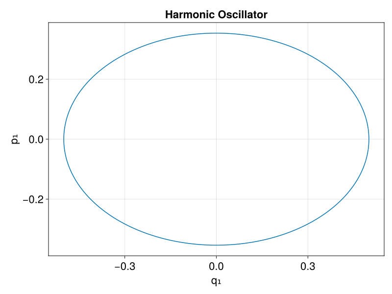
fig = lines(parent(sol.q[:,1]), parent(sol.p[:,1]);
    axis = (; xlabel = "q₁", ylabel = "p₁", title = "Harmonic Oscillator"),
    figure = (; size = (800,600), fontsize = 22))