Benchmarks
The package ships a benchmark suite (under benchmark/) for the one-layer GML variational integrator NonLinear_OneLayer_GML. It runs each of several test problems through a large grid of integrator configurations and records, for every case, whether the nonlinear solve converged, how accurate the result is, how much the energy drifts, how many nonlinear iterations it took, and how long it ran. The results are written to CSV, summarised in a markdown report, and visualised with a set of plots.
The suite has three goals:
- find which integrator-parameter configurations work well for each test problem;
- identify issues in the package that are detrimental to performance;
- identify robust solver strategies.
There is also a separate, narrower benchmark/oga_comparison.jl that compares the two OGA initial-guess variants; see the Orthogonal Greedy Algorithm page and benchmark/README.md.
What is swept
Each case integrates a problem for exactly 10 time steps; the time span is adapted per case as (0, 10·dt). The sweep spans, per problem:
| axis | meaning |
|---|---|
timestep dt | integration step size |
| precision | working floating-point type (Float16 / Float32 / Float64) |
R | Gauss–Legendre quadrature order |
S | number of hidden neurons (network width) |
| activation | ReLUᵏ (k = 2, 3, 4), ELU, GELU, or tanh |
| solver strategy | Newton with Static / Backtracking / StrongWolfe line search, or trust-region DogLeg |
λ | Jacobian regularization (regularization_factor) |
| initial guess | midpoint (IntegratorExtrapolation), Hermite (HermiteExtrapolation), or previous (NoExtrapolation) |
The test problems (from GeometricProblems.jl) are the harmonic oscillator, the pendulum (a degenerate two-component IODE — it has no lodeproblem), the double pendulum, and the Toda lattice with N = 16.
Modes
Each per-problem run file takes a mode — quick (default) or full — from its first command-line argument or from the GML_BENCH_PRESET environment variable.
| axis | full | quick |
|---|---|---|
dt | 0.01, 0.1, 1.0, 10.0 | 0.1, 1.0, 10.0 |
| precision | Float16, Float32, Float64 | Float64, Float32, Float16 |
R | 4, 8, 16 | 8 (16 for double pendulum & Toda) |
S | 4, 6, 8 | 4 (8 for double pendulum & Toda) |
| activation | ReLU², ReLU³, ReLU⁴, ELU, GELU, tanh | GELU, tanh |
| solver | Newton/{Static, Backtracking, StrongWolfe}, DogLeg | DogLeg |
λ | 0.0, 1e-7, 1e-5, 1e-3, 16√eps(T) | 16√eps(T) |
| initial guess | midpoint, Hermite, previous | midpoint |
max_iterations | 10000 | 100 |
quick is roughly 18 cases per problem (seconds to minutes each — the Toda lattice is the slowest because of its N = 16 state and larger network); full is on the order of tens of thousands of cases per problem (hours). Results are flushed to CSV per case, so an interrupted full run keeps its partial output.
The 16√eps(T) regularization scales the Jacobian-diagonal damping with the working precision: ≈2.4e-7 at Float64, ≈5.5e-3 at Float32, and 0.5 at Float16. The last is large and tends to over-damp half precision; note, however, that at half precision the ReLUᵏ basis is ill-conditioned and diverges independently of λ, whereas tanh still converges — the accuracy limit there is the precision, not the regularization.
Metrics
For each case the suite records:
- status —
ok, or a failure class (singular,diverged,nonfinite, or the short name of any other exception raised); ref_err— the relative max-norm error of the final state against a reference, which is aGauss(8)integration atFloat64using the smallest timestep in the sweep (over the same 10-step horizon);ham_drift— the maximum relative drift of the Hamiltonian over the run;iterations— the nonlinear-solver iteration count of the final step;solve_secs/total_secs— the summed nonlinear-solve time and the wall-clock time of the run.
Running
Instantiate the benchmark environment (it devs the package):
julia --project=benchmark -e 'using Pkg; Pkg.develop(PackageSpec(path=pwd())); Pkg.instantiate()'Run one or more problems (mode defaults to quick):
julia --project=benchmark benchmark/run_harmonic_oscillator.jl
julia --project=benchmark benchmark/run_pendulum.jl
julia --project=benchmark benchmark/run_double_pendulum.jl
julia --project=benchmark benchmark/run_toda_lattice.jl full   # full sweep
Each run writes benchmark/results/<problem>_<mode>.csv, a benchmark/results/<problem>_<mode>.md report, and PNG plots. Finally, aggregate every CSV present into a combined report:
julia --project=benchmark benchmark/report.jlwhich writes benchmark/results/onelayer_gml_benchmark.md. The reporting step reads the CSVs, so a report can be regenerated (or restyled) without re-running the sweep. All benchmark/results/ contents are git-ignored.
Outputs
The CSV has one row per case with the columns
problem, T, dt, steps, R, S, activation, solver, linesearch, initial_guess,
lambda, status, ref_err, ham_drift, iterations, solve_secs, total_secs
The markdown report contains a status breakdown, convergence/robustness tables (by solver strategy, initial-guess strategy, precision, and problem), the best configuration found per problem, and failure hot-spots. It embeds the plots:
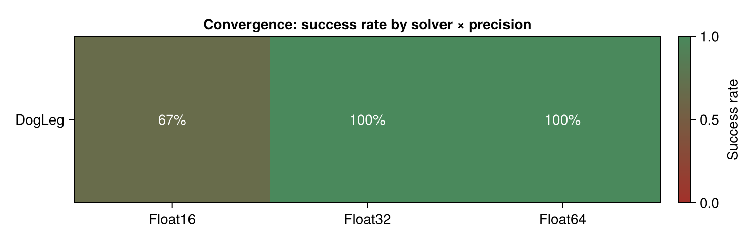
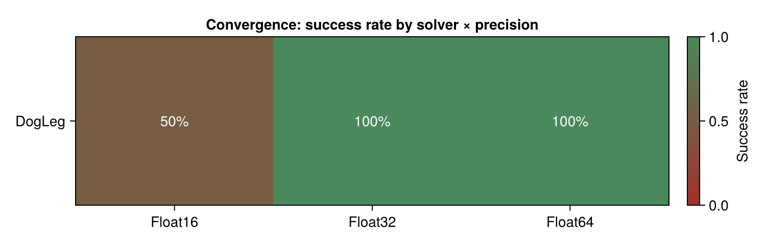
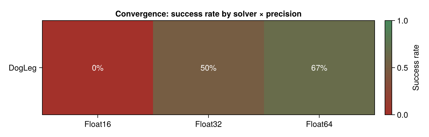
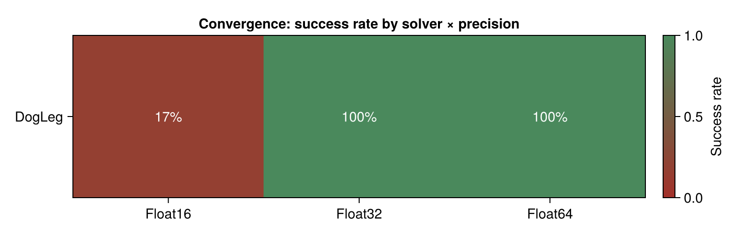
- convergence — success-rate bars per solver strategy, and a solver × precision heatmap (red = not converged, green = converged); the combined report also draws a success-rate bar per problem;
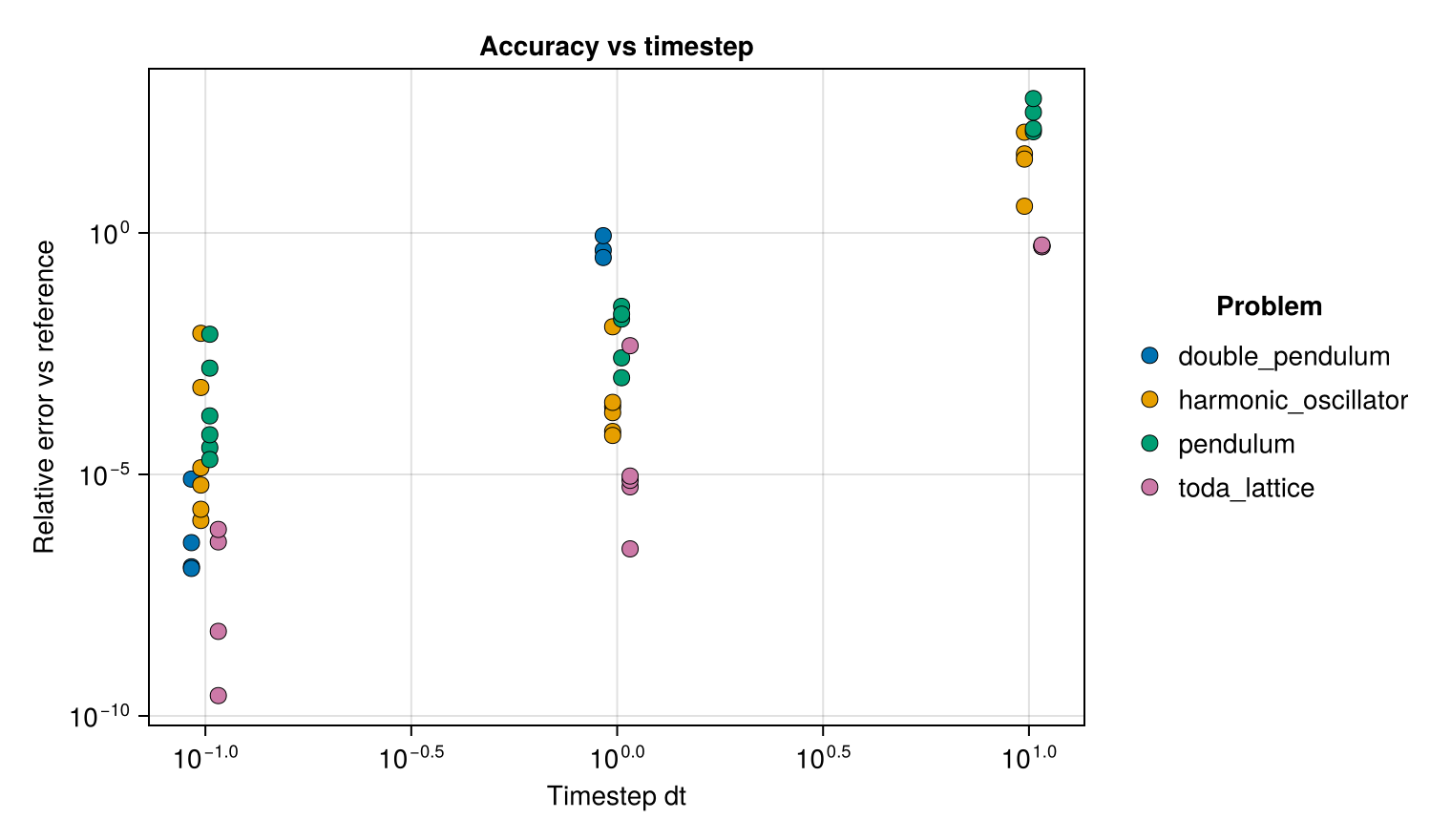
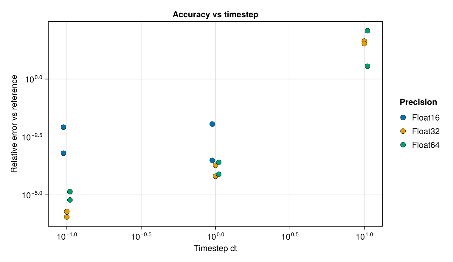
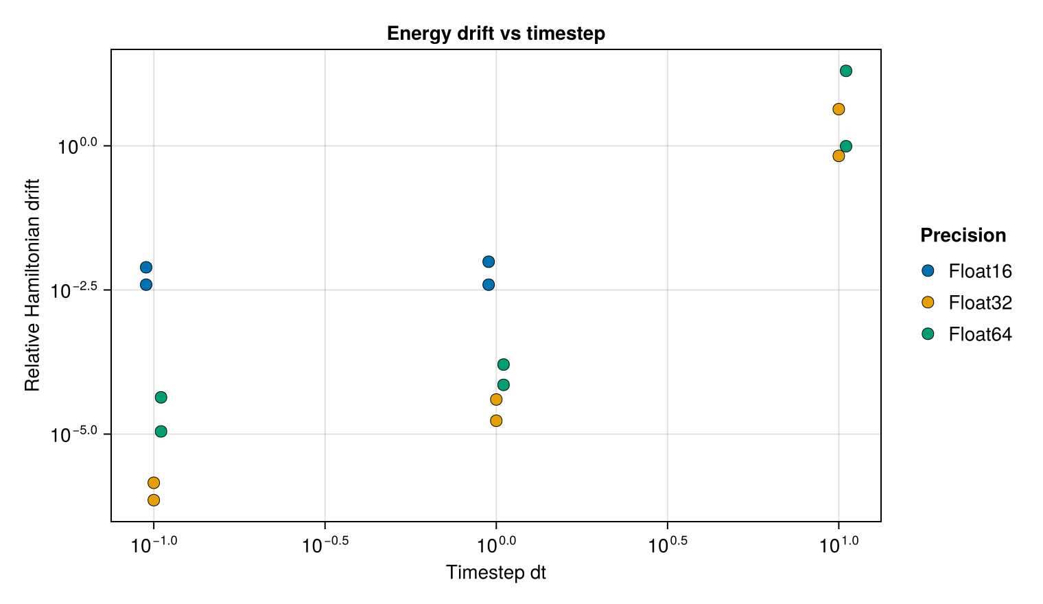
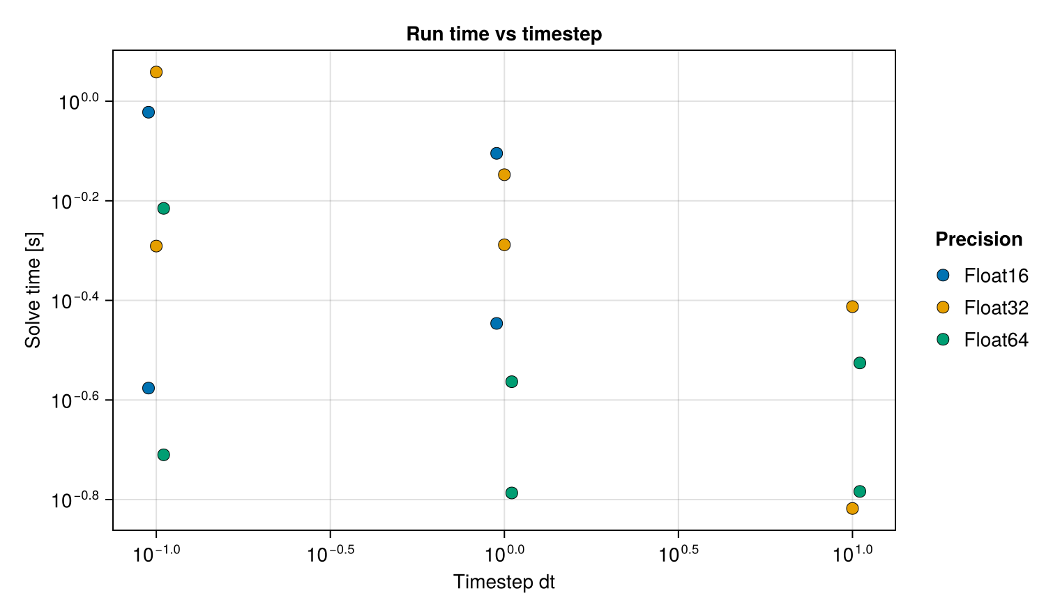
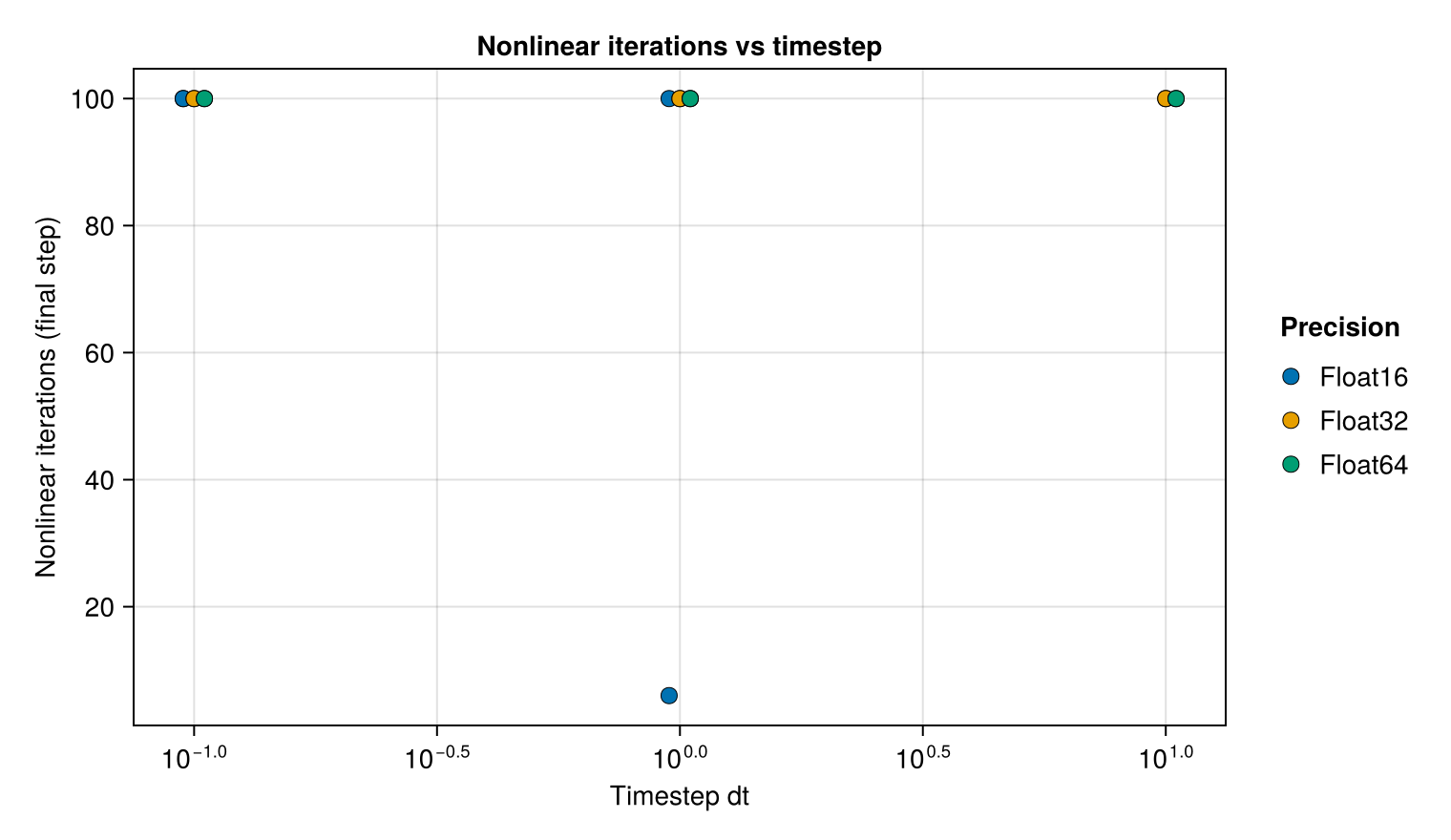
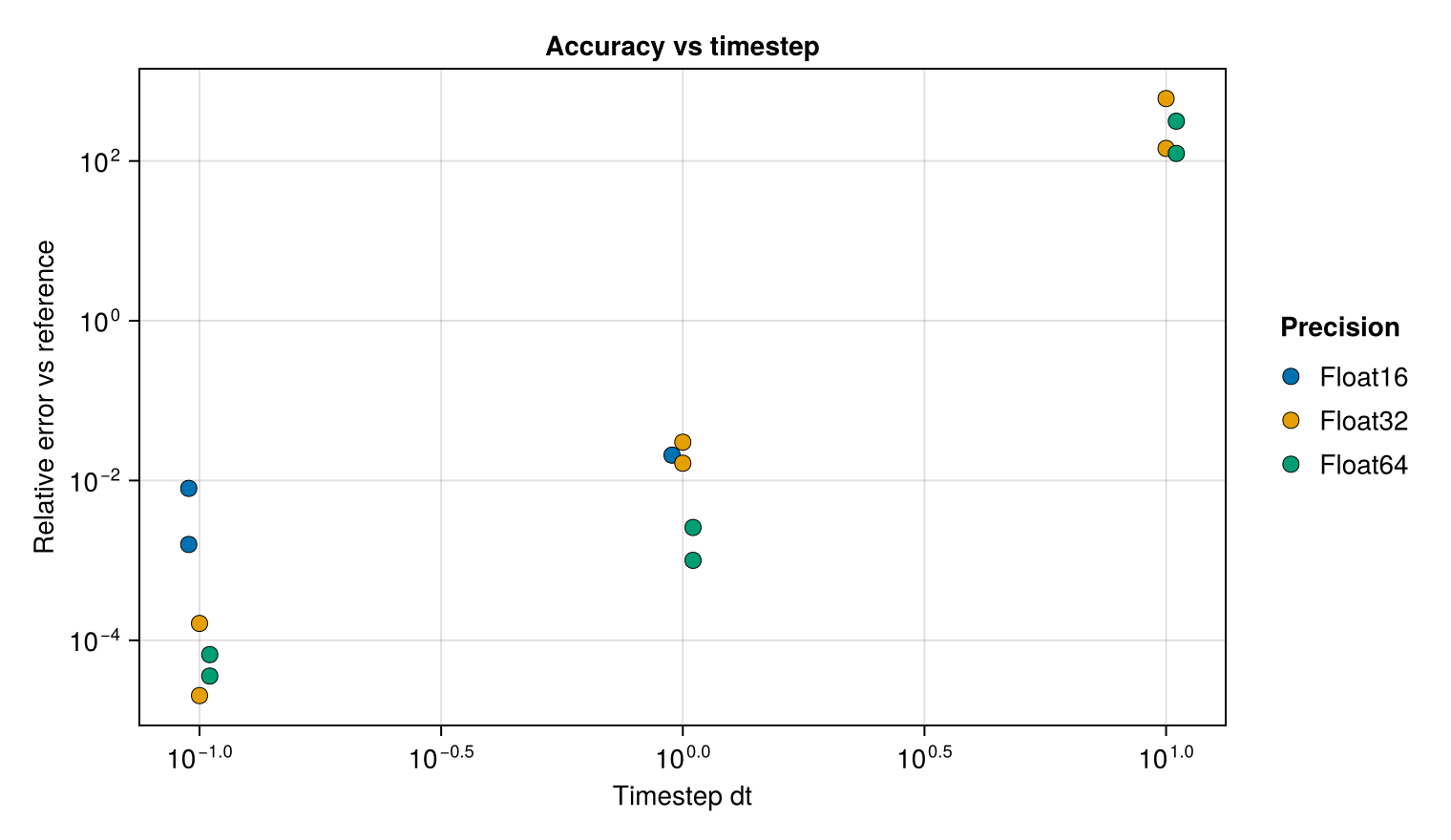
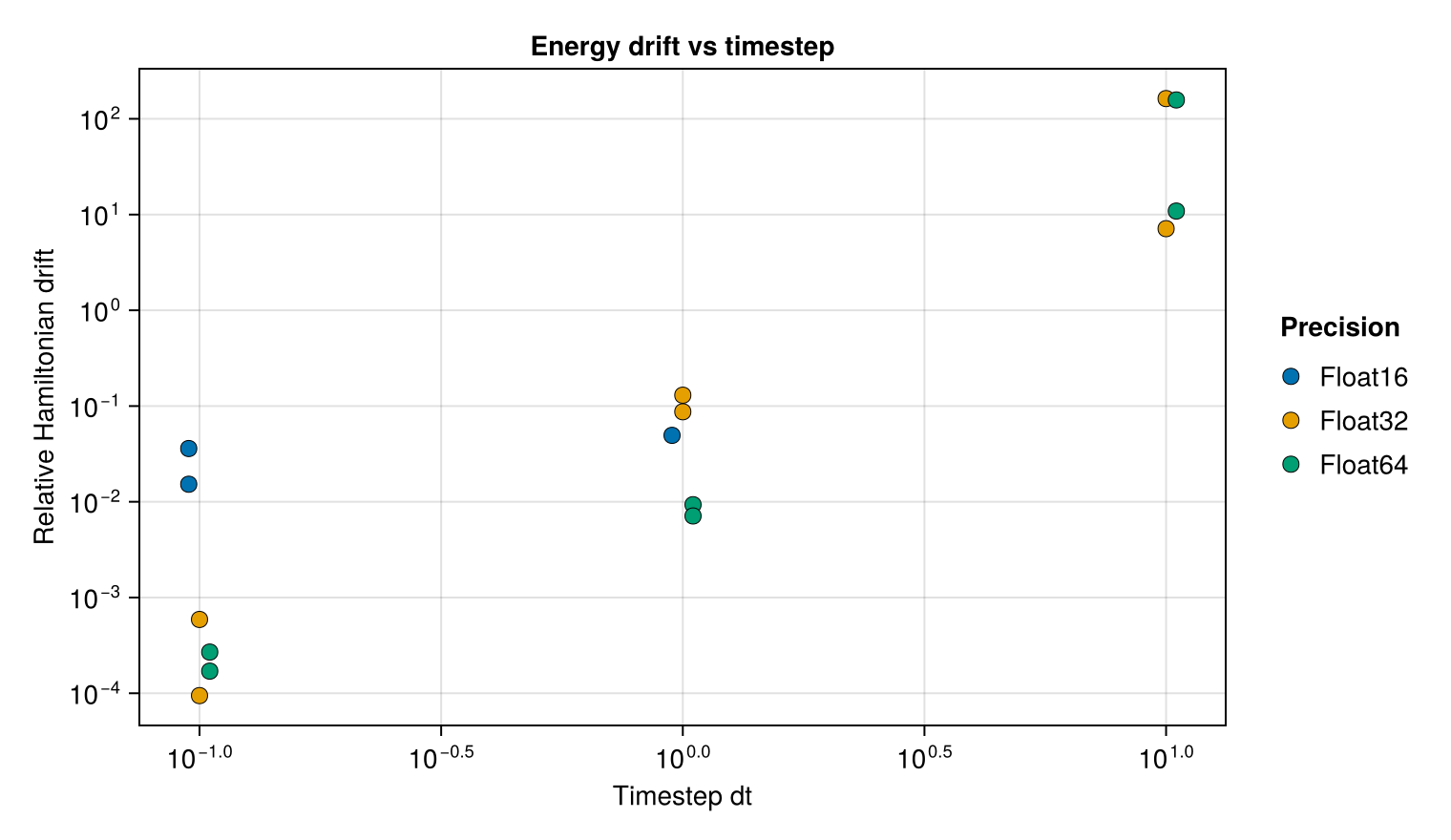
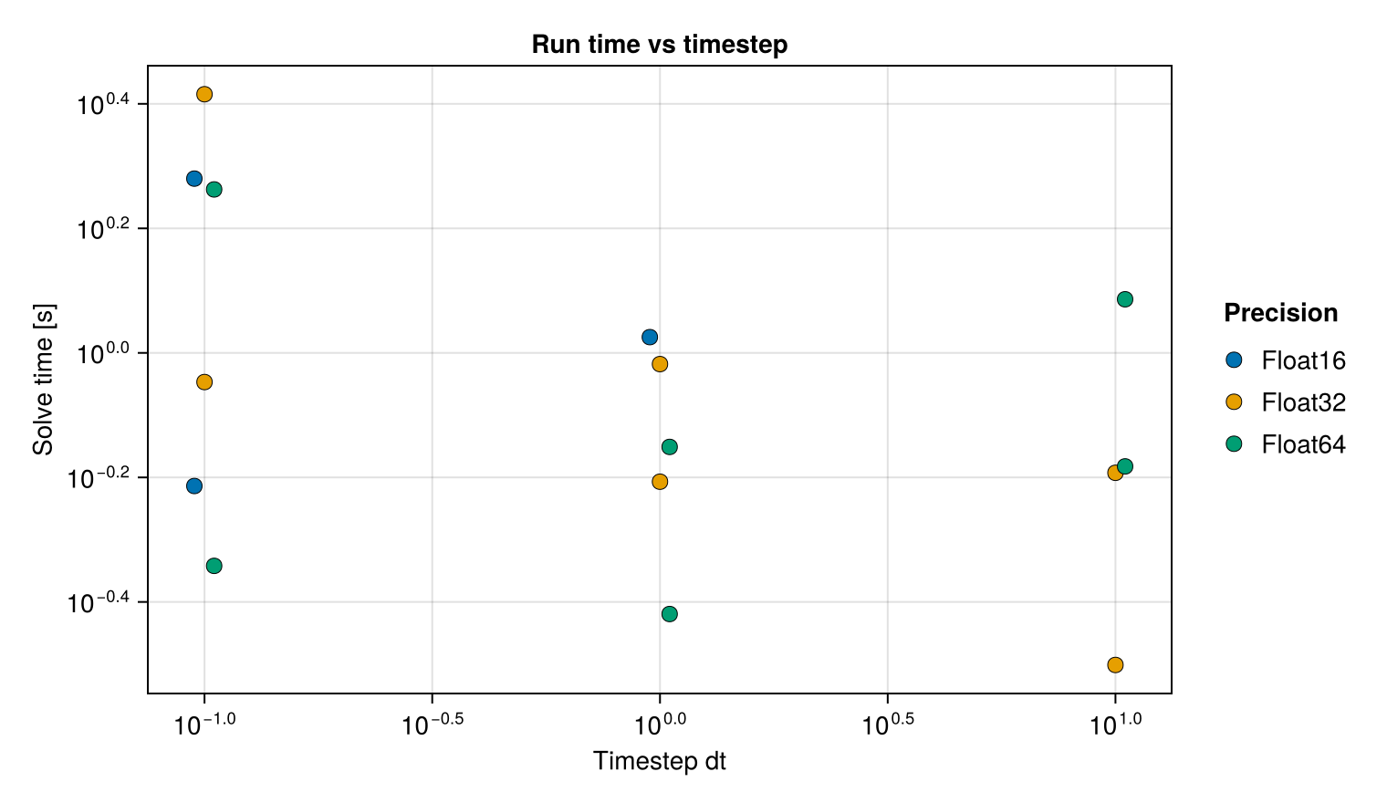
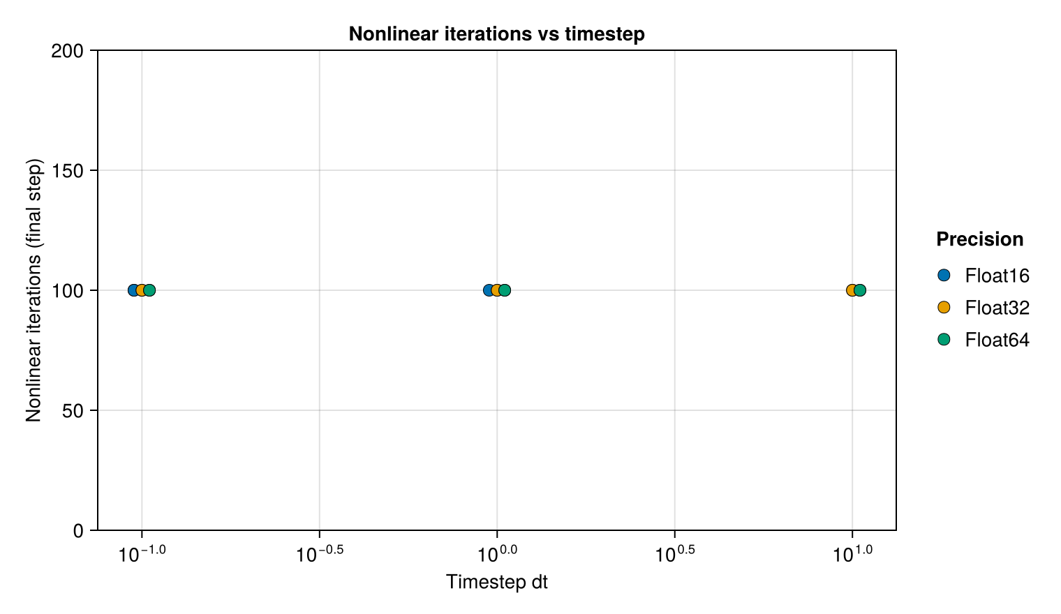
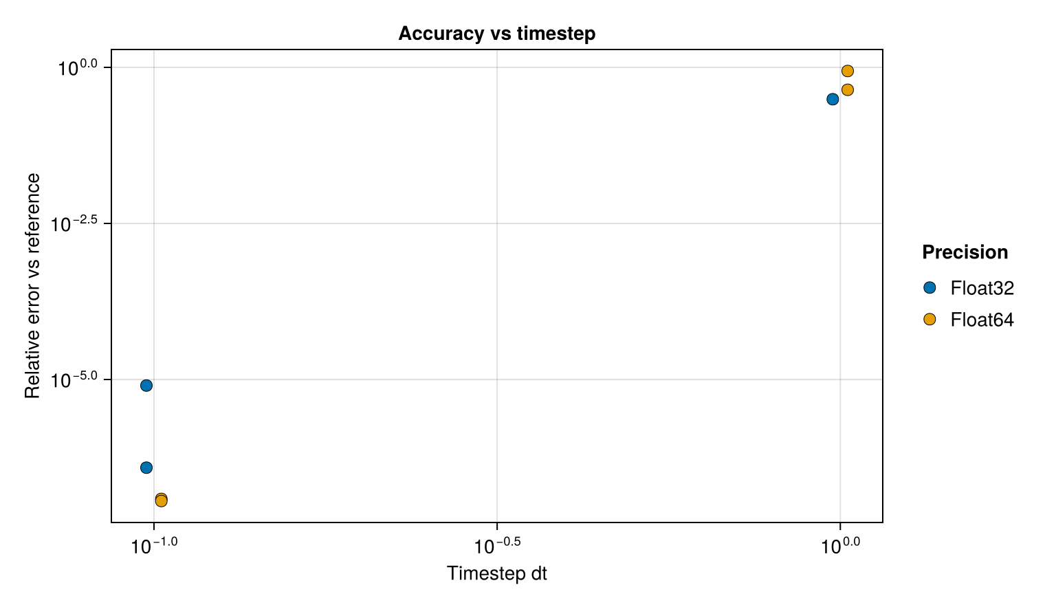
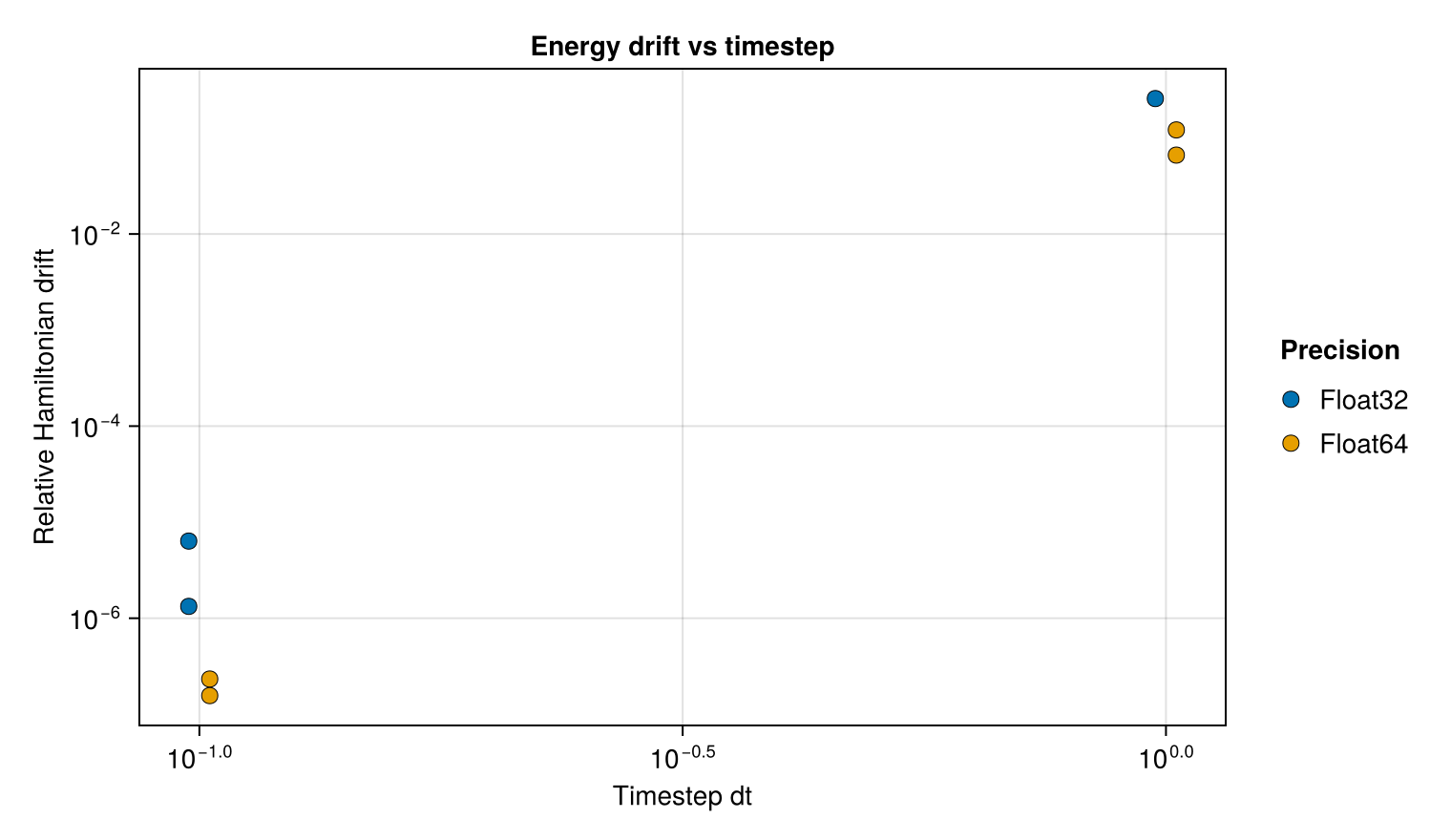
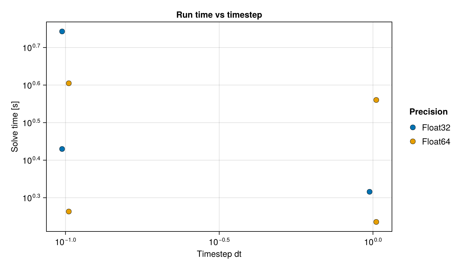
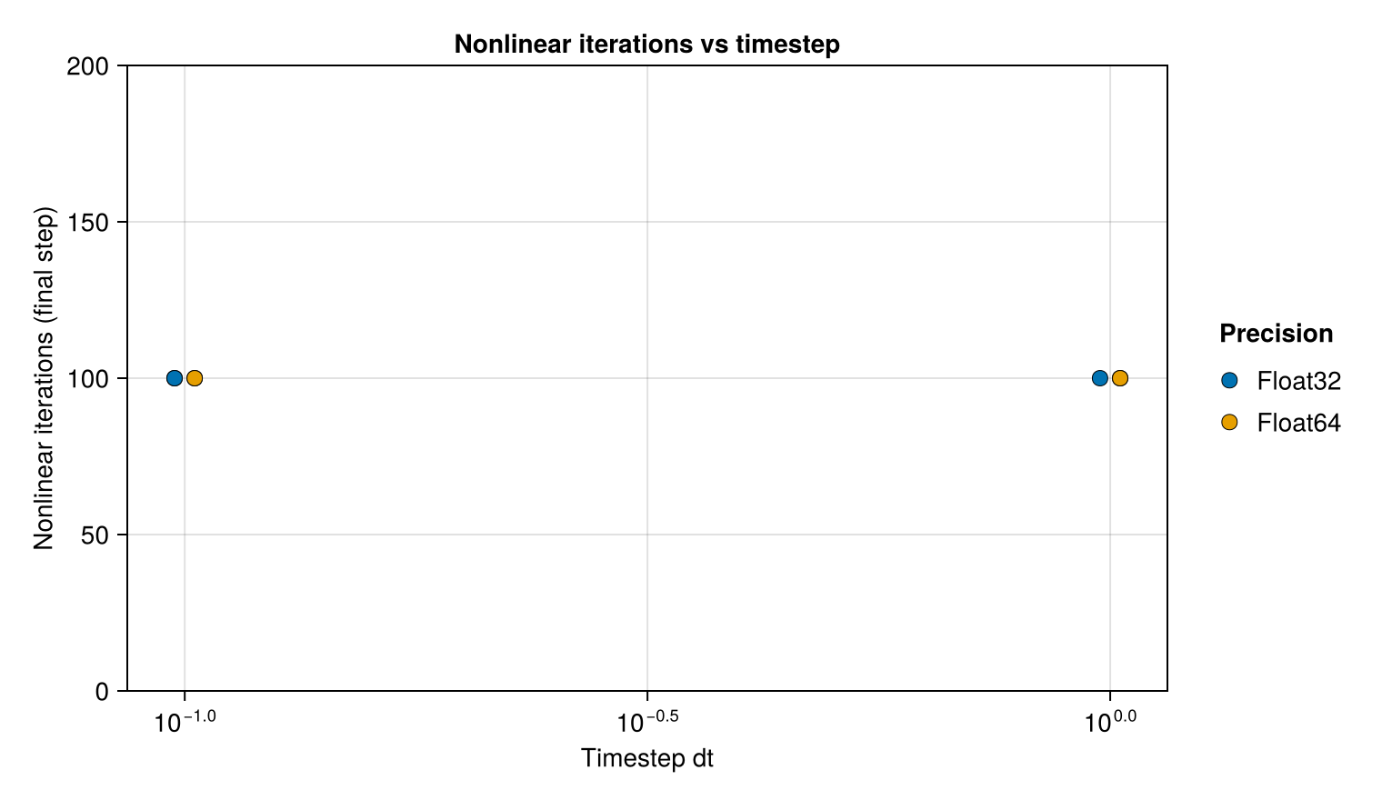
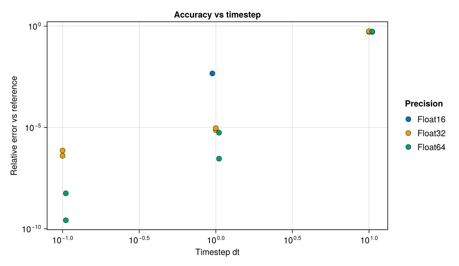
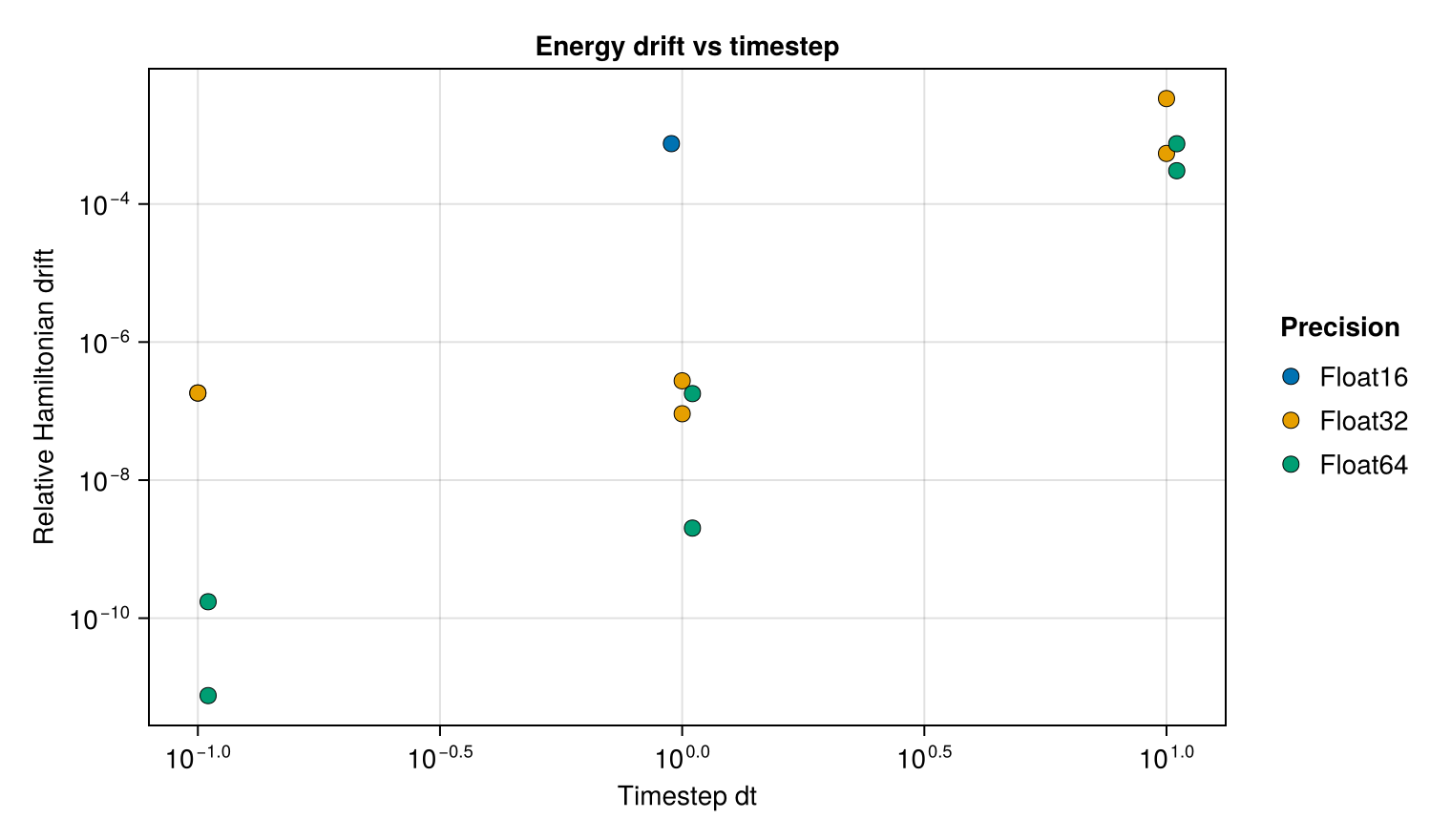
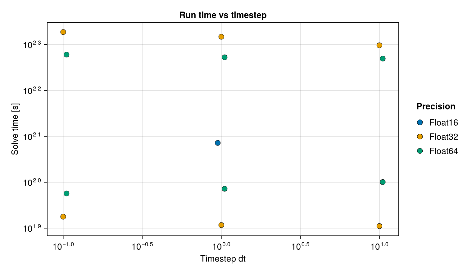
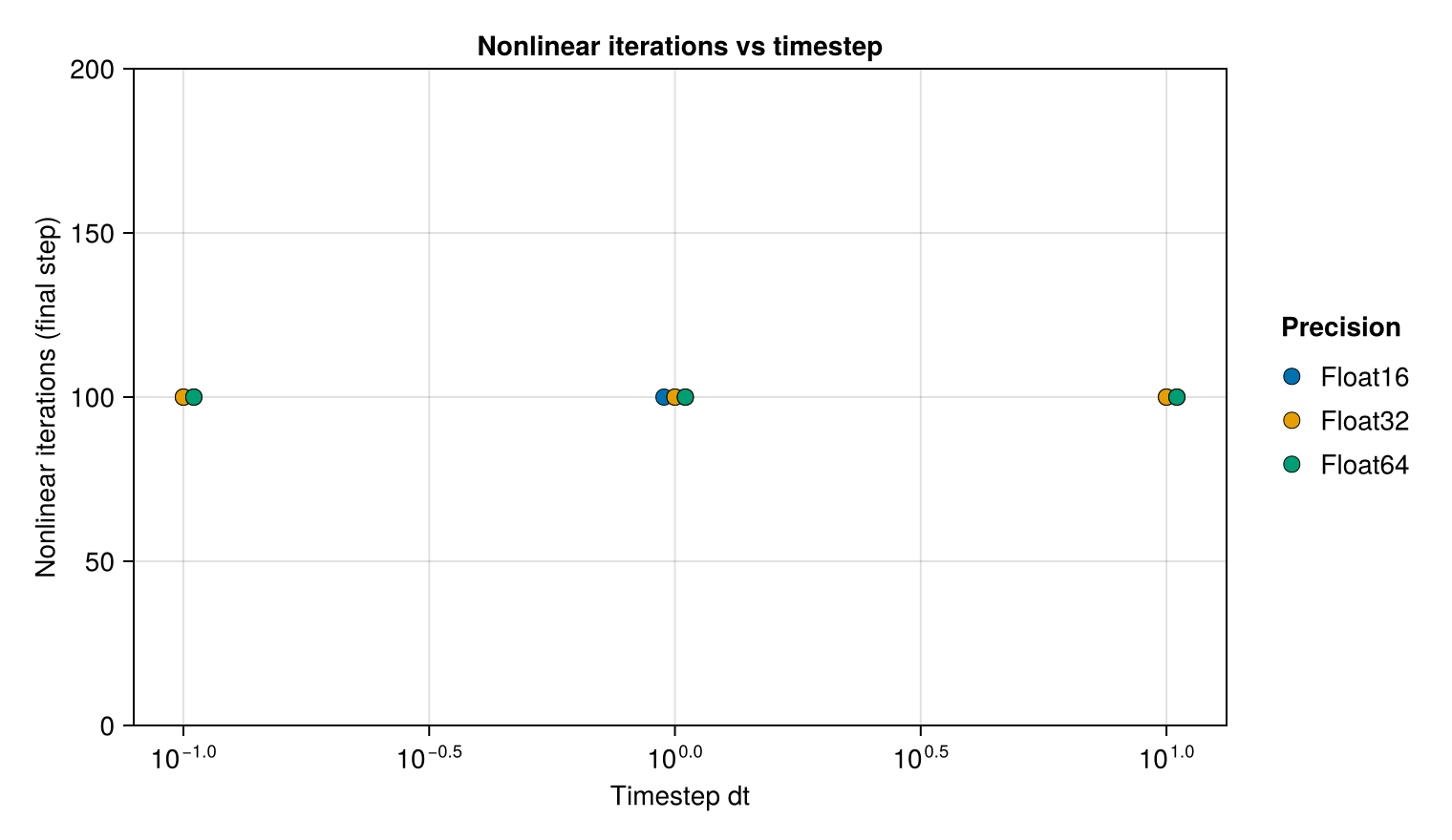
- accuracy, energy drift, run time, and nonlinear iterations — each as a scatter versus the timestep. A per-problem report colours the dots by precision; the combined report colours them by problem, so the four problems stay distinguishable.
Results
The figures on this page are not committed: they are regenerated at documentation-build time by a fresh quick run over the four problems (driven from docs/make.jl), so they track the current package. The narrative and tables are kept as an illustrative reference from one representative run — the numbers are not a fixed reference and may not match the freshly generated figures exactly. That run used the DogLeg solver, the midpoint initial guess, and the precision-scaled regularization λ = 16√eps(T).
Results are organised as a summary across all problems followed by one section per problem (harmonic oscillator, pendulum, double pendulum, Toda lattice). The summary scatters are coloured by problem; each per-problem section shows that problem's scatters coloured by precision.
Summary across all problems
Across the four problems (72 cases in the representative run), 48 converged. Convergence is dominated by precision: half precision is by far the least robust.
| precision | cases | converged | success | median ref_err | median ham_drift |
|---|---|---|---|---|---|
| Float16 | 24 | 5 | 21% | 7.15e-03 | 7.81e-03 |
| Float32 | 24 | 21 | 88% | 1.90e-04 | 1.04e-04 |
| Float64 | 24 | 22 | 92% | 2.22e-04 | 1.67e-04 |
Success rate broken down by problem, by solver strategy, and by solver × precision:
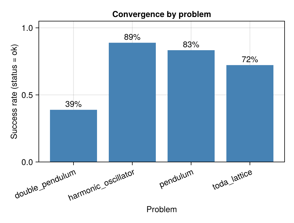
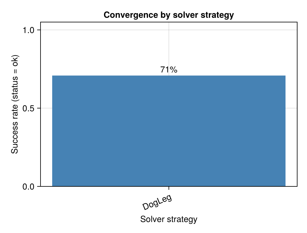
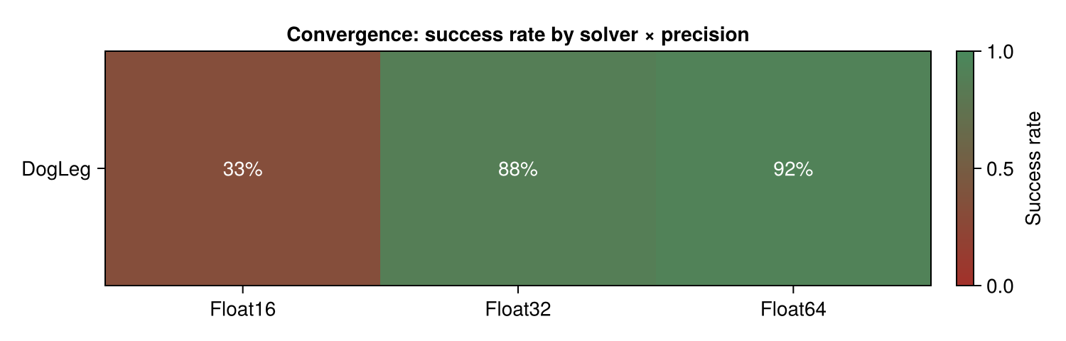
Accuracy, energy drift, run time and nonlinear-iteration counts versus the timestep, with all four problems overlaid and coloured by problem (each dot is one converged case). Accuracy and energy conservation degrade sharply as the timestep grows; at dt = 10 the 10-step horizon is far too coarse and the relative error is O(1).
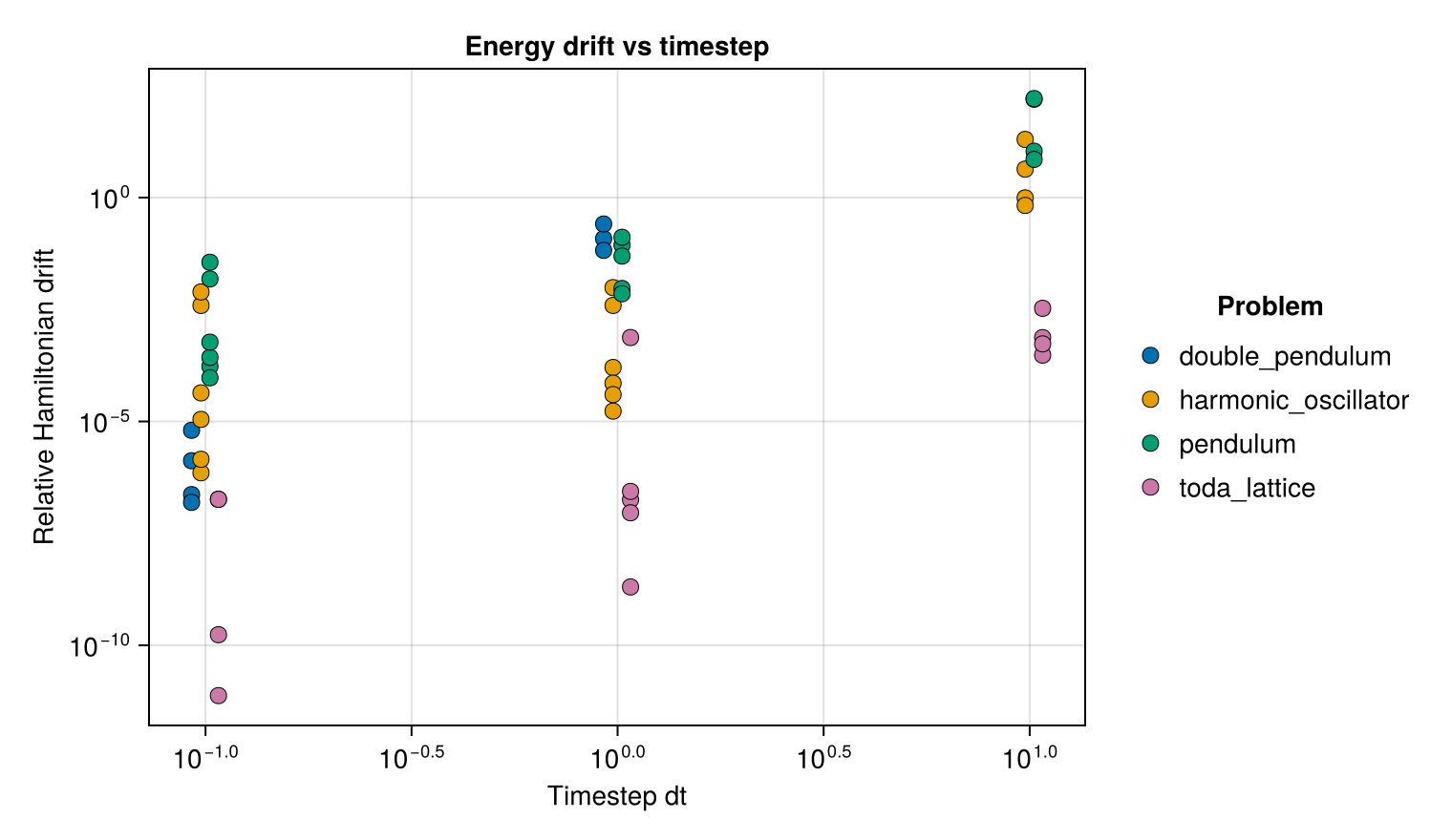
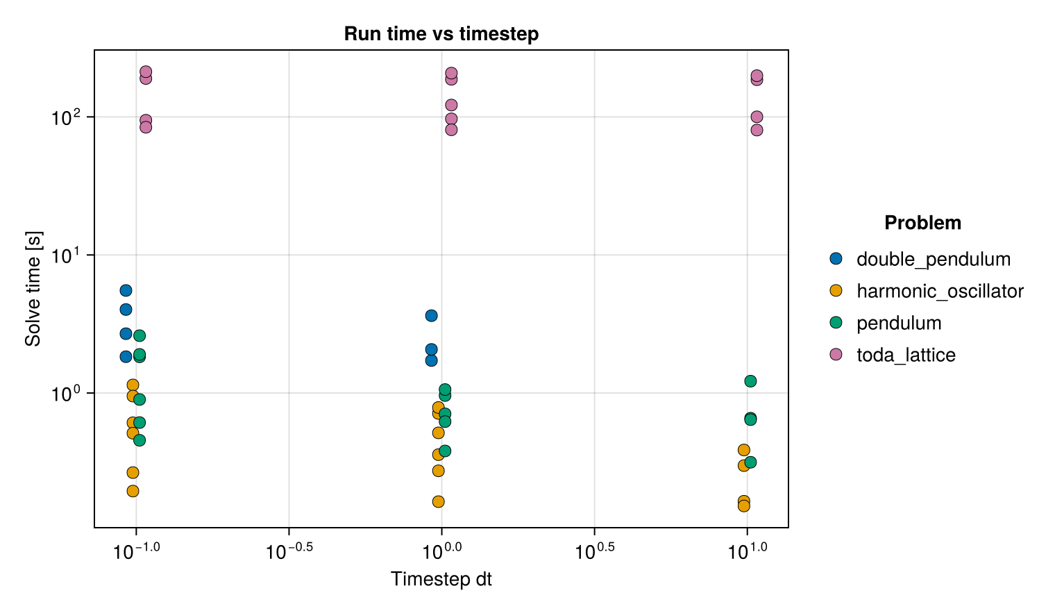
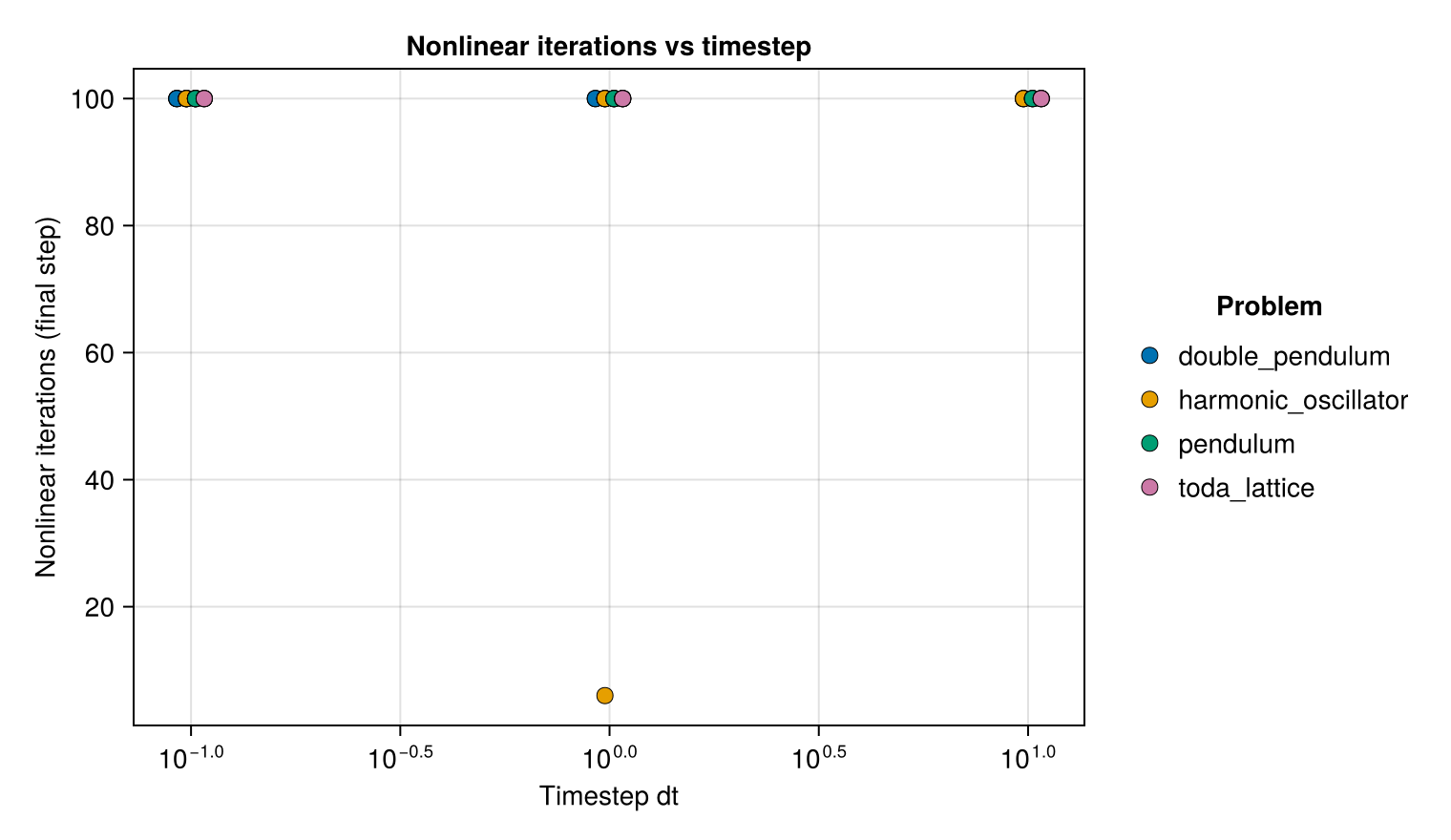
The best (lowest ref_err) converged configuration found for each problem:
| problem | best ref_err | T | dt | network | iguess / λ |
|---|---|---|---|---|---|
| harmonic_oscillator | 3.77e-13 | Float64 | 0.1 | R8 S4 ReLU³ | midpoint, λ=2.4e-7 |
| pendulum | 1.03e-07 | Float64 | 0.1 | R8 S4 ReLU³ | midpoint, λ=2.4e-7 |
| double_pendulum | 1.28e-07 | Float64 | 0.1 | R16 S8 tanh | midpoint, λ=2.4e-7 |
| toda_lattice | 1.55e-08 | Float64 | 0.1 | R16 S8 tanh | midpoint, λ=2.4e-7 |
The failures concentrate at half precision (across all timesteps) and at the largest timestep dt = 10 (across all precisions) — consistent with the accuracy plot.
Harmonic oscillator
The simplest test problem: a single linear oscillator. It reaches the best accuracy of the four (ref_err down to O(1e-13) at dt = 0.1, Float64), and the precision split is the clearest — Float64 and Float32 track each other closely while Float16 is limited by the working precision. Each dot below is a converged case, coloured by precision.
Pendulum
A degenerate two-component IODE (ϑ: p₁ = ml²q₂, p₂ = 0; it has no lodeproblem), included deliberately to stress the nonlinear solve. It is nonlinear and less accurate than the harmonic oscillator, and its half-precision cases are the most fragile.
Double pendulum
A four-dimensional chaotic system. Quick mode uses a larger network (R = 16, S = 8) than the two simple problems; tanh gives the best accuracy here.
Toda lattice (N = 16)
The largest problem, with a 16-dimensional state and a correspondingly larger network (R = 16, S = 8 in quick mode). It is the slowest to run — its run-time scatter sits above the other three problems in the summary.
Extending
To add a problem, copy one of the run_*.jl files and supply a build_prob(T, timespan, timestep) closure returning an AbstractProblemIODE at element type T, plus a hamiltonian(t, q, p, params) closure; then call run_sweep. Per-problem axis overrides (as the double pendulum and Toda lattice use for R and S) are passed as the Rs / Ss keyword arguments to run_sweep. The shared engine, presets, and reporting live in benchmark/gml_benchmark_common.jl and benchmark/gml_report.jl.