Linesearches for Optimizers
In GeometricOptimizers we typically build the search direction by applying the inverse Hessian to the negative gradient. When starting at $x_k$ we take:
\[ p_k = -H_{x_k}^{-1}(\nabla_{x_k}f),\]
where $[H_{x_k}]_{ij} = \frac{\partial^2{}f}{\partial{}x_i\partial{}x_j}\Big|_{x_k}$ is the Hessian. Note that we often use approximations of this Hessian in practice (such as the HessianBFGS).
The linesearch objective is then built as
\[f^\mathrm{ls}(\alpha) = f(x_k + \alpha{}p_k).\]
For manifolds [8] defining a Hessian, equivalently to defining a gradient, requires a Riemannian metric and the associated Levi-Civita connection $\nabla$:
\[\mathrm{Hess}(f) := \nabla\nabla{}f = \nabla{}df \in \Gamma(T^*\mathcal{M}\otimes{}T^*\mathcal{M}).\]
For specific vector fields $\xi, \eta \in \Gamma(T\mathcal{M})$ we can write this as:
\[\langle \mathrm{Hess}(f)[\xi], \eta \rangle = \xi(\eta{}f) - (\nabla_\xi\eta)f.\]
Example
We look at the following example:
f(x::Union{T, Vector{T}}) where {T<:Number} = exp.(x) .* (x .^ 3 .- 5x .+ 2x) .+ 2one(T)
f!(y::AbstractVector{T}, x::AbstractVector{T}) where {T} = y .= f.(x)
F!(y::AbstractVector{T}, x::AbstractVector{T}, params) where {T} = f!(y, x)
F! (generic function with 1 method)We hence use linesearch_problem not for a SimpleSolvers.NewtonSolver, but for an Optimizer:
# `f` has an inflection point at `x ≈ .75`; the starting point lies to the right of it, so the
# Hessian is positive definite here and the Newton direction descends. See the warning below.
x₀ = [.9, 1., 1.1]
x = copy(x₀)
obj = OptimizerProblem(sum∘f, x₀)
grad = GradientAutodiff{Float64}(obj.F, length(x₀))
_cache = NewtonOptimizerCache(x₀)
state = NewtonOptimizerState(x₀)
hess = HessianAutodiff(obj, x₀)
update!(state, grad, x₀)
update!(_cache, state, grad, hess, x₀)
params = (x = state.x, state = state)
# the retraction is how a trial step is taken; on an `AbstractVector` like this one it is
# never consulted, but `linesearch_problem` needs it for the manifold case
ls_obj = linesearch_problem(obj, grad, _cache, Cayley())

fˡˢ(alpha) = ls_obj.F(alpha, params)
∂fˡˢ∂α(alpha) = ls_obj.D(alpha, params)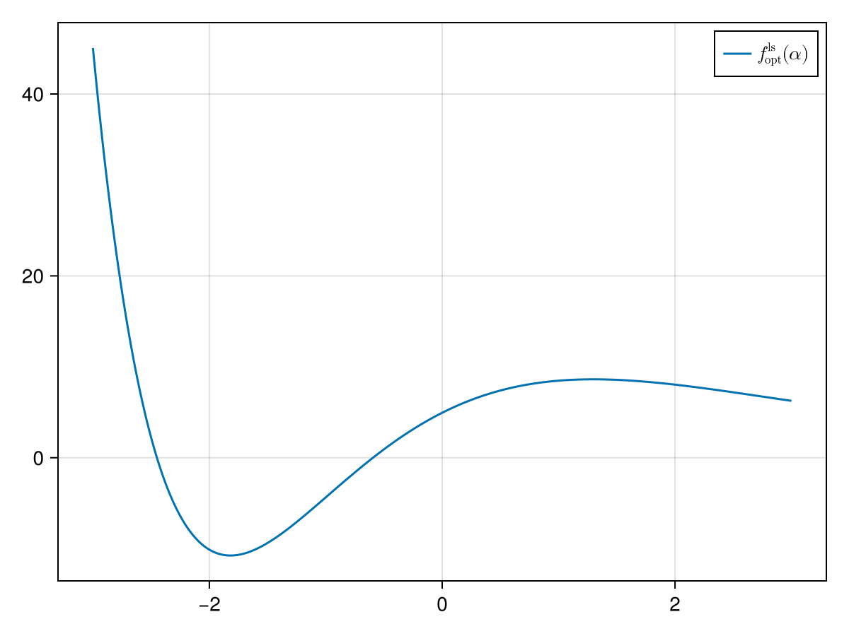
Note the different shape of the line search problem in the case of the optimizer, especially that the line search problem can take negative values in this case!
A line search only ever returns a step $\alpha \geq 0$, so it can minimise $f^\mathrm{ls}$ only along a direction that descends. The test is $\nabla{}f\cdot{}p < 0$, and the Newton direction $p = -H^{-1}\nabla{}f$ passes it wherever $H$ is positive definite. Started from $x_0 = (0, 0.1, 0.2)$ — where $f''$ is about $-6$ in every component — this same construction gives $(f^\mathrm{ls})'(0) = +6.45$ and a concave $f^\mathrm{ls}$, which no quadratic fit can minimise; SimpleSolvers.Quadratic reports LINESEARCH_NO_DESCENT on it without taking a single trial step. Inside a solve that case never reaches the search: ensure_descent! substitutes the steepest-descent direction for the step. Building the direction by hand, as this page does, skips that safeguard, so the starting point has to supply the descent itself.
We now again want to find the minimum with quadratic line search and repeat the procedure above:
p₀ = fˡˢ(0.)-10.199644290158965p₁ = ∂fˡˢ∂α(0.)-10.570505836469346params = (x = state.x, state = state)
# the second return value: the bracket's *right* end. The first is the left end, which is the
# fixed point the bracketing starts from, i.e. `0.` here — and `p₂` divides by `α₀²`.
α₀ = bracket_minimum_with_fixed_point(ls_obj, params, 0.)[2]
y = fˡˢ(α₀)
p₂ = (y - p₀ - p₁*α₀) / α₀^2
p(α) = p₀ + p₁ * α + p₂ * α^2
α₁ = -p₁ / (2p₂)0.30046625010630035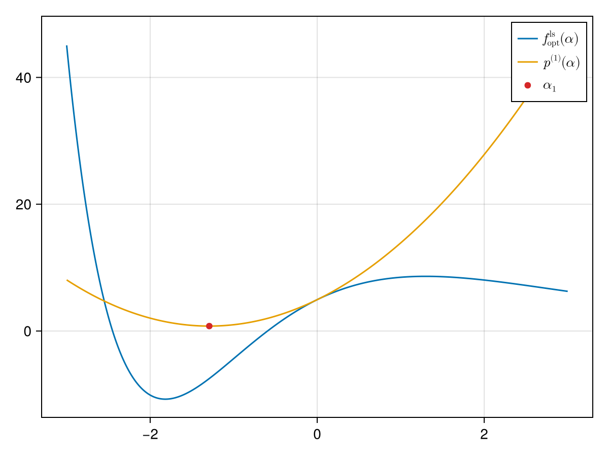
We now again move the original $x$ in the Newton direction with step length $\alpha_1$:
(sum∘f)(x)-10.199644290158965compute_new_iterate!(x, α₁, direction(_cache))3-element Vector{Float64}:
1.2335451033290121
1.1502331250531501
1.168294739245007(sum∘f)(x)-12.498846303050588