Symmetric, Skew-Symmetric and Triangular Matrices

Among the special arrays implemented in GeometricOptimizers SymmetricMatrix, SkewSymMatrix, StrictlyUpperTriangular and StrictlyLowerTriangular are the most common ones and similar implementations can also be found in other libraries; LinearAlgebra.jl has an implementation of a symmetric matrix called Symmetric for example. The versions of these matrices in GeometricOptimizers are however more memory efficient as they only store as many parameters as are necessary, i.e. $n(n+1)/2$ for the symmetric matrix and $n(n-1)/2$ for the other three. In addition, GeometricMachineLearning implements matrix and tensor multiplication for these matrices so that they work in parallel on GPU; see Tensors there. We here give an overview of elementary custom matrices that are implemented in GeometricOptimizers. More involved matrices are the so-called global tangent spaces.

Custom Matrices

GeometricOptimizers has two types of triangular matrices. The first one is StrictlyUpperTriangular:

\[U = \begin{pmatrix} 0 & a_{12} & \cdots & a_{1n} \\ 0 & \ddots & & a_{2n} \\ \vdots & \ddots & \ddots & \vdots \\ 0 & \cdots & 0 & 0 \end{pmatrix}.\]

And the second one is StrictlyLowerTriangular:

\[L = \begin{pmatrix} 0 & 0 & \cdots & 0 \\ a_{21} & \ddots & & \vdots \\ \vdots & \ddots & \ddots & \vdots \\ a_{n1} & \cdots & a_{n(n-1)} & 0 \end{pmatrix}.\]

adjoint swaps between the two: L' is a StrictlyUpperTriangular and U' is a StrictlyLowerTriangular. That swap is built around the same storage vector rather than a copy, so parent(L') === parent(L) holds and writing into L' also writes into L. Reusing the storage transposes without conjugating, so that swap is bound to a real element type; a complex one falls through to LinearAlgebra's lazy Adjoint, which conjugates and does not alias.

An instance of SkewSymMatrix can be written as $A = L - L^T$ or $A = U^T - U$:

\[A = \begin{pmatrix} 0 & - a_{21} & \cdots & - a_{n1} \\ a_{21} & \ddots & & \vdots \\ \vdots & \ddots & \ddots & \vdots \\ a_{n1} & \cdots & a_{n(n-1)} & 0 \end{pmatrix}.\]

And lastly a SymmetricMatrix:

\[B = \begin{pmatrix} a_{11} & a_{21} & \cdots & a_{n1} \\ a_{21} & \ddots & & \vdots \\ \vdots & \ddots & \ddots & \vdots \\ a_{n1} & \cdots & a_{n(n-1)} & a_{nn} \end{pmatrix}.\]

Note that any matrix $M\in\mathbb{R}^{n\times{}n}$ can be written

\[M = \frac{1}{2}(M - M^T) + \frac{1}{2}(M + M^T),\]

where the first part of this matrix is skew-symmetric and the second part is symmetric. This is also how the constructors for SkewSymMatrix and SymmetricMatrix are designed. Consider an arbitrary matrix:

M = [1; 2; 3;; 4; 5; 6;; 7; 8; 9]

3×3 Matrix{Int64}:
 1  4  7
 2  5  8
 3  6  9

Calling SkewSymMatrix on $M$ is equivalent to doing $M \to \frac{1}{2}(M - M^T)$:

A = SkewSymMatrix(M)

3×3 SkewSymMatrix{Float64, Vector{Float64}}:
  0.0   1.0  2.0
 -1.0   0.0  1.0
 -2.0  -1.0  0.0

And calling SymmetricMatrix on $M$ is equivalent to doing $M \to \frac{1}{2}(M + M^T)$:

B = SymmetricMatrix(M)

3×3 SymmetricMatrix{Float64, Vector{Float64}}:
 1.0  3.0  5.0
 3.0  5.0  7.0
 5.0  7.0  9.0

We can further confirm the identity above:

M  ≈ A + B

true

Note that for StrictlyLowerTriangular and StrictlyUpperTriangular no projection step is involved, which means that if we start with a matrix of type AbstractMatrix{Int64} we will end up with a matrix that is also of type AbstractMatrix{Int64}. The type changes however when we call SkewSymMatrix and SymmetricMatrix:

(typeof(A) <: AbstractMatrix{Int64}, typeof(B) <: AbstractMatrix{Int64})

(false, false)

For the triangular matrices:

U = StrictlyUpperTriangular(M)
L = StrictlyLowerTriangular(M)
(typeof(U) <: AbstractMatrix{Int64}, typeof(L) <: AbstractMatrix{Int64})

(true, true)

How are Special Matrices Stored?

The following image demonstrates how a skew-symmetric matrix is stored in GeometricOptimizers:

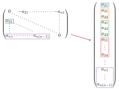
So what is stored internally is a vector of size $n(n-1)/2$ for the skew-symmetric matrix and the triangular matrices, and a vector of size $n(n+1)/2$ for the symmetric matrix.

Sample Random Matrices

We can sample a random skew-symmetric matrix:

A = rand(SkewSymMatrix, 3)

3×3 SkewSymMatrix{Float64, Vector{Float64}}:
 0.0       -0.521214  -0.586807
 0.521214   0.0       -0.890879
 0.586807   0.890879   0.0

and then access the vector:

A.S

3-element Vector{Float64}:
 0.521213795535383
 0.5868067574533484
 0.8908786980927811

This is equivalent to sampling a vector and then assigning a matrix^[1]:

S = rand(3 * (3 - 1) ÷ 2)
SkewSymMatrix(S, 3)

3×3 SkewSymMatrix{Float64, Vector{Float64}}:
 0.0       -0.521214  -0.586807
 0.521214   0.0       -0.890879
 0.586807   0.890879   0.0

These special matrices are what the layers of GeometricMachineLearning are parametrized by: SympNets, the volume-preserving transformer and the linear symplectic transformer all use one or more of them. That package also batches them over the third axis of a tensor, with mat_tensor_mul and tensor_mat_mul; see Tensors there.

Where a sampled array lands, and what it holds

Every owned type has one allocator convention, zeros([backend,] X{T}, dims...) and rand([rng,] [backend,] X{T}, dims...): the backend defaults to CPU(), a bare X means default_eltype of the backend, and rng defaults to Random.default_rng(). A manifold has rand only. So a call comes in four shapes, by whether it names a backend and whether it names an element type. The shape decides both answers, and it decides them the same way for the structured matrices above, for the manifolds and for the horizontal lifts:

The third and fourth shapes place on the host without saying so, and that is deliberate. They mirror Base, where zeros(Float32, 3) is a host array and nothing about the call suggests otherwise; these types present as AbstractMatrix, so zeros(SkewSymMatrix{Float32}, n) should read as the Array case does. A host placement also cannot quietly corrupt a device computation: mixing one with a device array throws at the first arithmetic — *, +, -, mul! and add! refuse a pair on two backends with an ArgumentError that names both — so the loud failure already gives the guarantee that making these shapes take a backend would buy. copyto! and assign! are the deliberate exception, because they are the transfer: moving a host-built structured matrix onto a device is what they exist for.

The second shape is the only one where the package decides something the caller did not, which is why the choice is a stated rule rather than a literal: Float64 on the host, Float32 on a device. See default_eltype for why each value is what it is, and note that a backend being able to hold a Float64 is not one of the reasons.

The first shape has a rule of its own, in the other direction: an element type the caller names and the backend cannot hold is refused, not narrowed. The backend's own allocation refuses it, so rand(MetalBackend(), SkewSymMatrix{Float64}, n) and rand(MetalBackend(), StiefelManifold{Float64}, N, n) both raise Metal's ErrorException, whose message names Float64. A narrowed result would have a different type from the one asked for, which is exactly what naming the element type rules out.

None of this reaches an allocation the package makes for itself. zero, similar, _zero and _similar all take an instance, so the backend and the element type both come from the argument and there is nothing to default — which is what every optimizer cache and every state allocates through. A parameter set on a device stays there.

Arithmetic and broadcasting on a device

A product, a sum, a difference and a mul! between two of these matrices, or between one of them and a plain array, run on the backend of their operands: the structured matrices, the horizontal lifts, the manifold points, StiefelProjection and the adjoints of each. None of them reads an entry at a time, which a device does not serve.

A broadcast does. These matrices define no broadcast style, so A .+ 1 or f.(A) reads A through getindex, and on a device that raises Scalar indexing is disallowed. Broadcast over the storage instead — parent(A) for the structured matrices, Y.A for a manifold point — and rebuild the matrix around the result where its structure still holds. A manifold point is left without a broadcast style on purpose: a broadcast over a point returns a plain array, because its result is in general not on the manifold.

Why the storage matters here

Because these types keep only their free parameters, they are also what an optimizer has to be able to update — and the generic array methods cannot do it: three of the four have no setindex! for an elementwise operation to broadcast through, similar has to preserve the type rather than widen to a dense Matrix, and $n(n\pm1)/2$ numbers do not reshape back to $n \times n$. See VectorStorageMatrix for the methods that make them usable as optimizer parameters.

The same storage is what a flat parameter vector and a saved file have to hold, for the same reason: $n(n\pm1)/2$ numbers are the whole content of one of these matrices, and the $n^2$ entries of the dense interface are neither the right length nor, for three of the four types, writable at all. NeuralNetworkParameters asks a leaf type for exactly that relation, through its freeparameters/rebuild pair, and loading it alongside this package brings in an extension that answers for all three families here — these matrices, the manifolds, and the horizontal lifts. Flattening, differentiating and saving a parameter set that contains them therefore needs no case per type in the package doing the training.

A gradient of one of these matrices has two forms, and they are not equal. The natural cotangent is a matrix of the same structure: ChainRulesCore.ProjectTo gives it for a dense cotangent $\bar{A} = \partial L/\partial A$, as the Frobenius projection $\frac{1}{2}(\bar{A} \pm \bar{A}^T)$. Automatic differentiation can add two natural cotangents and project the sum again, because the projection is linear and idempotent. The storage gradient $\partial L/\partial S$ is what the flat parameter vector and forward-mode differentiation give. An off-diagonal entry of a SymmetricMatrix appears twice in the matrix, so its storage gradient is $\bar{A}_{ij} + \bar{A}_{ji}$, twice the natural cotangent; the diagonal entries agree. For a SkewSymMatrix every storage entry is $\bar{A}_{ij} - \bar{A}_{ji}$, again twice the natural cotangent. The triangular types store each entry once, so the two forms agree.

This package converts the one to the other where a cotangent becomes a parameter gradient, through the storage_gradient hook of NeuralNetworkParameters. So Zygote.gradient(L, ps) for a parameter set ps gives the storage gradient at every leaf, and the flat gradient of a parameter set is $\partial L/\partial S$ — however often the loss uses a leaf, and whether or not it also reads the leaf as a dense matrix. The horizontal lifts get the same conversion for their blocks.

Element types

These matrices, and the package as a whole, support real element types only. The storage of a SymmetricMatrix and a SkewSymMatrix describes $A^T = \pm A$, which is not a Hermitian structure for a complex $A$. A complex element type is not rejected, and some operations give a wrong answer for it.

Library functions

AbstractTriangular, StrictlyUpperTriangular, StrictlyLowerTriangular, SkewSymMatrix, SymmetricMatrix and VectorStorageMatrix. Their docstrings are on the reference page, where every docstring in the package is rendered once; the names above link to them.